Note
Go to the end to download the full example code.
STEPS nowcast#
This tutorial shows how to compute and plot an ensemble nowcast using Swiss radar data.
import matplotlib.pyplot as plt
import numpy as np

from datetime import datetime
from pprint import pprint
from pysteps import io, nowcasts, rcparams
from pysteps.motion.lucaskanade import dense_lucaskanade
from pysteps.postprocessing.ensemblestats import excprob
from pysteps.utils import conversion, dimension, transformation
from pysteps.visualization import plot_precip_field

# Set nowcast parameters
n_ens_members = 20
n_leadtimes = 6
seed = 24
Read precipitation field#
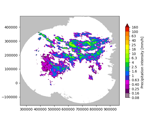
First thing, the sequence of Swiss radar composites is imported, converted and transformed into units of dBR.
date = datetime.strptime("201701311200", "%Y%m%d%H%M")
data_source = "mch"

# Load data source config
root_path = rcparams.data_sources[data_source]["root_path"]
path_fmt = rcparams.data_sources[data_source]["path_fmt"]
fn_pattern = rcparams.data_sources[data_source]["fn_pattern"]
fn_ext = rcparams.data_sources[data_source]["fn_ext"]
importer_name = rcparams.data_sources[data_source]["importer"]
importer_kwargs = rcparams.data_sources[data_source]["importer_kwargs"]
timestep = rcparams.data_sources[data_source]["timestep"]

# Find the radar files in the archive
fns = io.find_by_date(
    date, root_path, path_fmt, fn_pattern, fn_ext, timestep, num_prev_files=2
)

# Read the data from the archive
importer = io.get_method(importer_name, "importer")
R, _, metadata = io.read_timeseries(fns, importer, **importer_kwargs)

# Convert to rain rate
R, metadata = conversion.to_rainrate(R, metadata)

# Upscale data to 2 km to limit memory usage
R, metadata = dimension.aggregate_fields_space(R, metadata, 2000)

# Plot the rainfall field
plot_precip_field(R[-1, :, :], geodata=metadata)
plt.show()

# Log-transform the data to unit of dBR, set the threshold to 0.1 mm/h,
# set the fill value to -15 dBR
R, metadata = transformation.dB_transform(R, metadata, threshold=0.1, zerovalue=-15.0)

# Set missing values with the fill value
R[~np.isfinite(R)] = -15.0

# Nicely print the metadata
pprint(metadata)
/home/docs/checkouts/readthedocs.org/user_builds/pysteps/envs/stable/lib/python3.11/site-packages/pysteps/visualization/utils.py:439: UserWarning: cartopy package is required for the get_geogrid function but it is not installed. Ignoring geographical information.
  warnings.warn(
{'accutime': 5,
 'cartesian_unit': 'm',
 'institution': 'MeteoSwiss',
 'product': 'AQC',
 'projection': '+proj=somerc  +lon_0=7.43958333333333 +lat_0=46.9524055555556 '
               '+k_0=1 +x_0=600000 +y_0=200000 +ellps=bessel '
               '+towgs84=674.374,15.056,405.346,0,0,0,0 +units=m +no_defs',
 'threshold': -10.0,
 'timestamps': array([datetime.datetime(2017, 1, 31, 11, 50),
       datetime.datetime(2017, 1, 31, 11, 55),
       datetime.datetime(2017, 1, 31, 12, 0)], dtype=object),
 'transform': 'dB',
 'unit': 'mm/h',
 'x1': 255000.0,
 'x2': 965000.0,
 'xpixelsize': 2000,
 'y1': -160000.0,
 'y2': 480000.0,
 'yorigin': 'upper',
 'ypixelsize': 2000,
 'zerovalue': -15.0,
 'zr_a': 316.0,
 'zr_b': 1.5}
Deterministic nowcast with S-PROG#
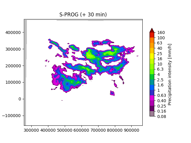
First, the motiong field is estimated using a local tracking approach based on the Lucas-Kanade optical flow. The motion field can then be used to generate a deterministic nowcast with the S-PROG model, which implements a scale filtering appraoch in order to progressively remove the unpredictable spatial scales during the forecast.
# Estimate the motion field
V = dense_lucaskanade(R)

# The S-PROG nowcast
nowcast_method = nowcasts.get_method("sprog")
R_f = nowcast_method(
    R[-3:, :, :],
    V,
    n_leadtimes,
    n_cascade_levels=6,
    precip_thr=-10.0,
)

# Back-transform to rain rate
R_f = transformation.dB_transform(R_f, threshold=-10.0, inverse=True)[0]

# Plot the S-PROG forecast
plot_precip_field(
    R_f[-1, :, :],
    geodata=metadata,
    title="S-PROG (+ %i min)" % (n_leadtimes * timestep),
)
plt.show()
Computing S-PROG nowcast
------------------------

Inputs
------
input dimensions: 320x355

Methods
-------
extrapolation:          semilagrangian
bandpass filter:        gaussian
decomposition:          fft
conditional statistics: no
probability matching:   cdf
FFT method:             numpy
domain:                 spatial

Parameters
----------
number of time steps:     6
parallel threads:         1
number of cascade levels: 6
order of the AR(p) model: 2
precip. intensity threshold: -10.0
Rain fraction is: 0.1692224178403756, while minimum fraction is 0.0
************************************************
* Correlation coefficients for cascade levels: *
************************************************
-----------------------------------------
| Level |     Lag-1     |     Lag-2     |
-----------------------------------------
| 1     | 0.999143      | 0.996712      |
-----------------------------------------
| 2     | 0.997163      | 0.987230      |
-----------------------------------------
| 3     | 0.989146      | 0.964330      |
-----------------------------------------
| 4     | 0.950503      | 0.860300      |
-----------------------------------------
| 5     | 0.811605      | 0.614387      |
-----------------------------------------
| 6     | 0.369440      | 0.192662      |
-----------------------------------------
****************************************
* AR(p) parameters for cascade levels: *
****************************************
------------------------------------------------------
| Level |    Phi-1     |    Phi-2     |    Phi-0     |
------------------------------------------------------
| 1     | 1.917687     | -0.919332    | 0.016286     |
------------------------------------------------------
| 2     | 1.854718     | -0.859995    | 0.038411     |
------------------------------------------------------
| 3     | 1.634281     | -0.652214    | 0.111381     |
------------------------------------------------------
| 4     | 1.375375     | -0.446998    | 0.277947     |
------------------------------------------------------
| 5     | 0.916986     | -0.129843    | 0.579261     |
------------------------------------------------------
| 6     | 0.345406     | 0.065056     | 0.927286     |
------------------------------------------------------
Starting nowcast computation.
Computing nowcast for time step 1... done.
Computing nowcast for time step 2... done.
Computing nowcast for time step 3... done.
Computing nowcast for time step 4... done.
Computing nowcast for time step 5... done.
Computing nowcast for time step 6... done.
/home/docs/checkouts/readthedocs.org/user_builds/pysteps/envs/stable/lib/python3.11/site-packages/pysteps/visualization/utils.py:439: UserWarning: cartopy package is required for the get_geogrid function but it is not installed. Ignoring geographical information.
  warnings.warn(
As we can see from the figure above, the forecast produced by S-PROG is a smooth field. In other words, the forecast variance is lower than the variance of the original observed field. However, certain applications demand that the forecast retain the same statistical properties of the observations. In such cases, the S-PROG forecasts are of limited use and a stochatic approach might be of more interest.
Stochastic nowcast with STEPS#
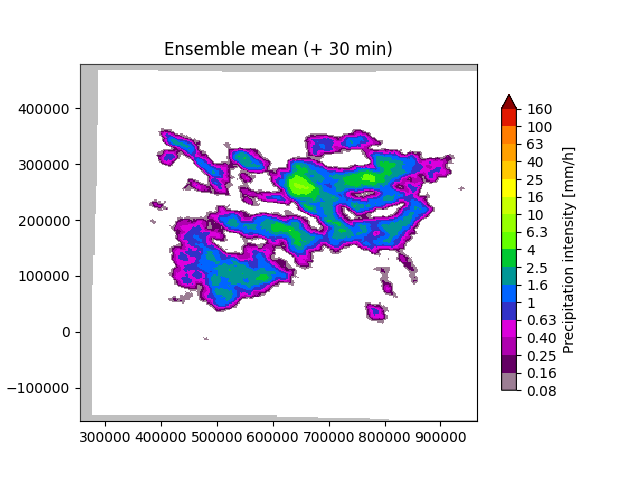
The S-PROG approach is extended to include a stochastic term which represents the variance associated to the unpredictable development of precipitation. This approach is known as STEPS (short-term ensemble prediction system).
# The STEPS nowcast
nowcast_method = nowcasts.get_method("steps")
R_f = nowcast_method(
    R[-3:, :, :],
    V,
    n_leadtimes,
    n_ens_members,
    n_cascade_levels=6,
    precip_thr=-10.0,
    kmperpixel=2.0,
    timestep=timestep,
    noise_method="nonparametric",
    vel_pert_method="bps",
    mask_method="incremental",
    seed=seed,
)

# Back-transform to rain rates
R_f = transformation.dB_transform(R_f, threshold=-10.0, inverse=True)[0]


# Plot the ensemble mean
R_f_mean = np.mean(R_f[:, -1, :, :], axis=0)
plot_precip_field(
    R_f_mean,
    geodata=metadata,
    title="Ensemble mean (+ %i min)" % (n_leadtimes * timestep),
)
plt.show()
Inputs validated and initialized successfully.
Computing STEPS nowcast
-----------------------

Inputs
------
input dimensions: 320x355
km/pixel:         2.0
time step:        5 minutes

Methods
-------
extrapolation:          semilagrangian
bandpass filter:        gaussian
decomposition:          fft
noise generator:        nonparametric
noise adjustment:       no
velocity perturbator:   bps
conditional statistics: no
precip. mask method:    incremental
probability matching:   cdf
FFT method:             numpy
domain:                 spatial

Parameters
----------
number of time steps:     6
ensemble size:            20
parallel threads:         1
number of cascade levels: 6
order of the AR(p) model: 2
velocity perturbations, parallel:      10.88,0.23,-7.68
velocity perturbations, perpendicular: 5.76,0.31,-2.72
precip. intensity threshold: -10.0
Nowcast components initialized successfully.
Rain fraction is: 0.1694630281690141, while minimum fraction is 0.0
Extrapolation complete and precipitation fields aligned.
************************************************
* Correlation coefficients for cascade levels: *
************************************************
-----------------------------------------
| Level |     Lag-1     |     Lag-2     |
-----------------------------------------
| 1     | 0.999143      | 0.996712      |
-----------------------------------------
| 2     | 0.997163      | 0.987230      |
-----------------------------------------
| 3     | 0.989146      | 0.964330      |
-----------------------------------------
| 4     | 0.950503      | 0.860300      |
-----------------------------------------
| 5     | 0.811605      | 0.614387      |
-----------------------------------------
| 6     | 0.369440      | 0.192662      |
-----------------------------------------
****************************************
* AR(p) parameters for cascade levels: *
****************************************
------------------------------------------------------
| Level |    Phi-1     |    Phi-2     |    Phi-0     |
------------------------------------------------------
| 1     | 1.917687     | -0.919332    | 0.016286     |
------------------------------------------------------
| 2     | 1.854718     | -0.859995    | 0.038411     |
------------------------------------------------------
| 3     | 1.634281     | -0.652214    | 0.111381     |
------------------------------------------------------
| 4     | 1.375375     | -0.446998    | 0.277947     |
------------------------------------------------------
| 5     | 0.916986     | -0.129843    | 0.579261     |
------------------------------------------------------
| 6     | 0.345406     | 0.065056     | 0.927286     |
------------------------------------------------------
AR model and noise applied to precipitation cascades.
Velocity perturbations initialized successfully.
Precipitation mask initialized successfully.
FFT objects initialized successfully.
Starting nowcast computation.
Computing nowcast for time step 1... done.
Computing nowcast for time step 2... done.
Computing nowcast for time step 3... done.
Computing nowcast for time step 4... done.
Computing nowcast for time step 5... done.
Computing nowcast for time step 6... done.
/home/docs/checkouts/readthedocs.org/user_builds/pysteps/envs/stable/lib/python3.11/site-packages/pysteps/visualization/utils.py:439: UserWarning: cartopy package is required for the get_geogrid function but it is not installed. Ignoring geographical information.
  warnings.warn(
The mean of the ensemble displays similar properties as the S-PROG forecast seen above, although the degree of smoothing also depends on the ensemble size. In this sense, the S-PROG forecast can be seen as the mean of an ensemble of infinite size.
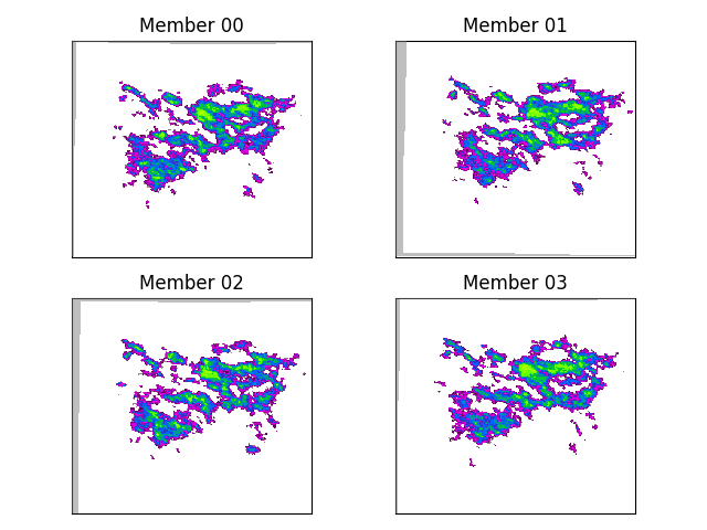
# Plot some of the realizations
fig = plt.figure()
for i in range(4):
    ax = fig.add_subplot(221 + i)
    ax = plot_precip_field(
        R_f[i, -1, :, :], geodata=metadata, colorbar=False, axis="off"
    )
    ax.set_title("Member %02d" % i)
plt.tight_layout()
plt.show()
/home/docs/checkouts/readthedocs.org/user_builds/pysteps/envs/stable/lib/python3.11/site-packages/pysteps/visualization/utils.py:439: UserWarning: cartopy package is required for the get_geogrid function but it is not installed. Ignoring geographical information.
  warnings.warn(
/home/docs/checkouts/readthedocs.org/user_builds/pysteps/envs/stable/lib/python3.11/site-packages/pysteps/visualization/utils.py:439: UserWarning: cartopy package is required for the get_geogrid function but it is not installed. Ignoring geographical information.
  warnings.warn(
/home/docs/checkouts/readthedocs.org/user_builds/pysteps/envs/stable/lib/python3.11/site-packages/pysteps/visualization/utils.py:439: UserWarning: cartopy package is required for the get_geogrid function but it is not installed. Ignoring geographical information.
  warnings.warn(
/home/docs/checkouts/readthedocs.org/user_builds/pysteps/envs/stable/lib/python3.11/site-packages/pysteps/visualization/utils.py:439: UserWarning: cartopy package is required for the get_geogrid function but it is not installed. Ignoring geographical information.
  warnings.warn(
As we can see from these two members of the ensemble, the stochastic forecast mantains the same variance as in the observed rainfall field. STEPS also includes a stochatic perturbation of the motion field in order to quantify the its uncertainty.
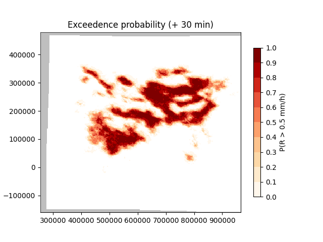
Finally, it is possible to derive probabilities from our ensemble forecast.
# Compute exceedence probabilities for a 0.5 mm/h threshold
P = excprob(R_f[:, -1, :, :], 0.5)

# Plot the field of probabilities
plot_precip_field(
    P,
    geodata=metadata,
    ptype="prob",
    units="mm/h",
    probthr=0.5,
    title="Exceedence probability (+ %i min)" % (n_leadtimes * timestep),
)
plt.show()

# sphinx_gallery_thumbnail_number = 5
/home/docs/checkouts/readthedocs.org/user_builds/pysteps/envs/stable/lib/python3.11/site-packages/pysteps/visualization/utils.py:439: UserWarning: cartopy package is required for the get_geogrid function but it is not installed. Ignoring geographical information.
  warnings.warn(
Total running time of the script: (0 minutes 10.482 seconds)