Data transformations

The statistics of intermittent precipitation rates are particularly non-Gaussian and display an asymmetric distribution bounded at zero. Such properties restrict the usage of well-established statistical methods that assume symmetric or Gaussian data.

A common workaround is to introduce a suitable data transformation to approximate a normal distribution.

In this example, we test the data transformation methods available in pysteps in order to obtain a more symmetric distribution of the precipitation data (excluding the zeros). The currently available transformations include the Box-Cox, dB, square-root and normal quantile transforms.

from datetime import datetime
import matplotlib.pyplot as plt
import numpy as np
from pysteps import io, rcparams
from pysteps.utils import conversion, transformation
from scipy.stats import skew

Read the radar input images

First, we will import the sequence of radar composites. You need the pysteps-data archive downloaded and the pystepsrc file configured with the data_source paths pointing to data folders.

# Selected case
date = datetime.strptime("201609281600", "%Y%m%d%H%M")
data_source = rcparams.data_sources["fmi"]

Load the data from the archive

root_path = data_source["root_path"]
path_fmt = data_source["path_fmt"]
fn_pattern = data_source["fn_pattern"]
fn_ext = data_source["fn_ext"]
importer_name = data_source["importer"]
importer_kwargs = data_source["importer_kwargs"]
timestep = data_source["timestep"]

# Get 1 hour of observations in the data archive
fns = io.archive.find_by_date(
    date, root_path, path_fmt, fn_pattern, fn_ext, timestep, num_next_files=11
)

# Read the radar composites
importer = io.get_method(importer_name, "importer")
Z, _, metadata = io.read_timeseries(fns, importer, **importer_kwargs)

# Keep only positive rainfall values
Z = Z[Z > metadata["zerovalue"]].flatten()

# Convert to rain rate
R, metadata = conversion.to_rainrate(Z, metadata)

Test data transformations

# Define method to visualize the data distribution with boxplots and plot the
# corresponding skewness
def plot_distribution(data, labels, skw):
    N = len(data)
    fig, ax1 = plt.subplots()
    ax2 = ax1.twinx()

    ax2.plot(np.arange(N + 2), np.zeros(N + 2), ":r")
    ax1.boxplot(data, labels=labels, sym="", medianprops={"color": "k"})

    ymax = []
    for i in range(N):
        y = skw[i]
        x = i + 1
        ax2.plot(x, y, "*r", ms=10, markeredgecolor="k")
        ymax.append(np.max(data[i]))

    # ylims
    ylims = np.percentile(ymax, 50)
    ax1.set_ylim((-1 * ylims, ylims))
    ylims = np.max(np.abs(skw))
    ax2.set_ylim((-1.1 * ylims, 1.1 * ylims))

    # labels
    ax1.set_ylabel(r"Standardized values [$\sigma$]")
    ax2.set_ylabel(r"Skewness []", color="r")
    ax2.tick_params(axis="y", labelcolor="r")

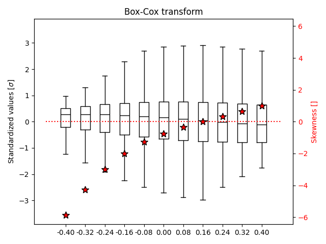
Box-Cox transform

The Box-Cox transform is a well-known power transformation introduced by Box and Cox (1964). In its one-parameter version, the Box-Cox transform takes the form T(x) = ln(x) for lambda = 0, or T(x) = (x**lambda - 1)/lambda otherwise.

To find a suitable lambda, we will experiment with a range of values and select the one that produces the most symmetric distribution, i.e., the lambda associated with a value of skewness closest to zero. To visually compare the results, the transformed data are standardized.

data = []
labels = []
skw = []

# Test a range of values for the transformation parameter Lambda
Lambdas = np.linspace(-0.4, 0.4, 11)
for i, Lambda in enumerate(Lambdas):
    R_, _ = transformation.boxcox_transform(R, metadata, Lambda)
    R_ = (R_ - np.mean(R_)) / np.std(R_)
    data.append(R_)
    labels.append("{0:.2f}".format(Lambda))
    skw.append(skew(R_))  # skewness

# Plot the transformed data distribution as a function of lambda
plot_distribution(data, labels, skw)
plt.title("Box-Cox transform")
plt.tight_layout()
plt.show()

# Best lambda
idx_best = np.argmin(np.abs(skw))
Lambda = Lambdas[idx_best]

print("Best parameter lambda: %.2f\n(skewness = %.2f)" % (Lambda, skw[idx_best]))

Best parameter lambda: 0.16
(skewness = 0.02)

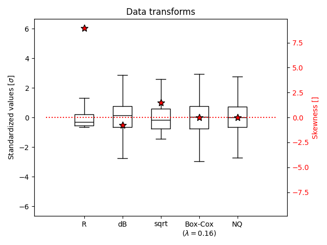
Compare data transformations

data = []
labels = []
skw = []

Rain rates

First, let’s have a look at the original rain rate values.

data.append((R - np.mean(R)) / np.std(R))
labels.append("R")
skw.append(skew(R))

dB transform

We transform the rainfall data into dB units: 10*log(R)

R_, _ = transformation.dB_transform(R, metadata)
data.append((R_ - np.mean(R_)) / np.std(R_))
labels.append("dB")
skw.append(skew(R_))

Square-root transform

Transform the data using the square-root: sqrt(R)

R_, _ = transformation.sqrt_transform(R, metadata)
data.append((R_ - np.mean(R_)) / np.std(R_))
labels.append("sqrt")
skw.append(skew(R_))

Box-Cox transform

We now apply the Box-Cox transform using the best parameter lambda found above.

R_, _ = transformation.boxcox_transform(R, metadata, Lambda)
data.append((R_ - np.mean(R_)) / np.std(R_))
labels.append("Box-Cox\n($\lambda=$%.2f)" % Lambda)
skw.append(skew(R_))

Normal quantile transform

At last, we apply the empirical normal quantile (NQ) transform as described in Bogner et al (2012).

R_, _ = transformation.NQ_transform(R, metadata)
data.append((R_ - np.mean(R_)) / np.std(R_))
labels.append("NQ")
skw.append(skew(R_))

By plotting all the results, we can notice first of all the strongly asymmetric distribution of the original data (R) and that all transformations manage to reduce its skewness. Among these, the Box-Cox transform (using the best parameter lambda) and the normal quantile (NQ) transform provide the best correction. Despite not producing a perfectly symmetric distribution, the square-root (sqrt) transform has the strong advantage of being defined for zeros, too, while all other transformations need an arbitrary rule for non-positive values.

plot_distribution(data, labels, skw)
plt.title("Data transforms")
plt.tight_layout()
plt.show()