Note
Go to the end to download the full example code.
Extrapolation nowcast#
This tutorial shows how to compute and plot an extrapolation nowcast using Finnish radar data.
from datetime import datetime
import matplotlib.pyplot as plt
import numpy as np
from pprint import pprint
from pysteps import io, motion, nowcasts, rcparams, verification
from pysteps.utils import conversion, transformation
from pysteps.visualization import plot_precip_field, quiver
Read the radar input images#
First, we will import the sequence of radar composites. You need the pysteps-data archive downloaded and the pystepsrc file configured with the data_source paths pointing to data folders.
# Selected case
date = datetime.strptime("201609281600", "%Y%m%d%H%M")
data_source = rcparams.data_sources["fmi"]
n_leadtimes = 12
Load the data from the archive#
root_path = data_source["root_path"]
path_fmt = data_source["path_fmt"]
fn_pattern = data_source["fn_pattern"]
fn_ext = data_source["fn_ext"]
importer_name = data_source["importer"]
importer_kwargs = data_source["importer_kwargs"]
timestep = data_source["timestep"]
# Find the input files from the archive
fns = io.archive.find_by_date(
date, root_path, path_fmt, fn_pattern, fn_ext, timestep, num_prev_files=2
)
# Read the radar composites
importer = io.get_method(importer_name, "importer")
Z, _, metadata = io.read_timeseries(fns, importer, **importer_kwargs)
# Convert to rain rate
R, metadata = conversion.to_rainrate(Z, metadata)
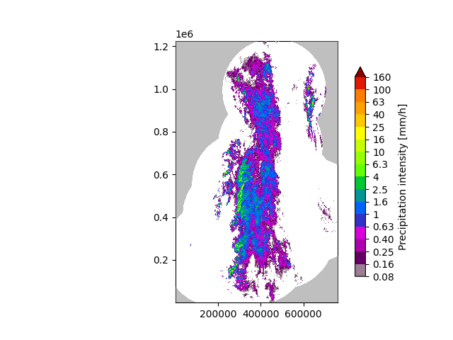
# Plot the rainfall field
plot_precip_field(R[-1, :, :], geodata=metadata)
plt.show()
# Store the last frame for plotting it later later
R_ = R[-1, :, :].copy()
# Log-transform the data to unit of dBR, set the threshold to 0.1 mm/h,
# set the fill value to -15 dBR
R, metadata = transformation.dB_transform(R, metadata, threshold=0.1, zerovalue=-15.0)
# Nicely print the metadata
pprint(metadata)
/home/docs/checkouts/readthedocs.org/user_builds/pysteps/envs/stable/lib/python3.11/site-packages/pysteps/visualization/utils.py:439: UserWarning: cartopy package is required for the get_geogrid function but it is not installed. Ignoring geographical information.
  warnings.warn(
{'accutime': 5.0,
 'cartesian_unit': 'm',
 'institution': 'Finnish Meteorological Institute',
 'projection': '+proj=stere  +lon_0=25E +lat_0=90N +lat_ts=60 +a=6371288 '
               '+x_0=380886.310 +y_0=3395677.920 +no_defs',
 'threshold': -10.0,
 'timestamps': array([datetime.datetime(2016, 9, 28, 15, 50),
       datetime.datetime(2016, 9, 28, 15, 55),
       datetime.datetime(2016, 9, 28, 16, 0)], dtype=object),
 'transform': 'dB',
 'unit': 'mm/h',
 'x1': 0.0049823258887045085,
 'x2': 759752.2852757066,
 'xpixelsize': 999.674053,
 'y1': 0.009731985162943602,
 'y2': 1225544.6588913496,
 'yorigin': 'upper',
 'ypixelsize': 999.62859,
 'zerovalue': -15.0,
 'zr_a': 223.0,
 'zr_b': 1.53}
Compute the nowcast#
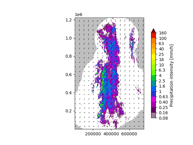
The extrapolation nowcast is based on the estimation of the motion field, which is here performed using a local tracking approach (Lucas-Kanade). The most recent radar rainfall field is then simply advected along this motion field in oder to produce an extrapolation forecast.
# Estimate the motion field with Lucas-Kanade
oflow_method = motion.get_method("LK")
V = oflow_method(R[-3:, :, :])

# Extrapolate the last radar observation
extrapolate = nowcasts.get_method("extrapolation")
R[~np.isfinite(R)] = metadata["zerovalue"]
R_f = extrapolate(R[-1, :, :], V, n_leadtimes)

# Back-transform to rain rate
R_f = transformation.dB_transform(R_f, threshold=-10.0, inverse=True)[0]

# Plot the motion field
plot_precip_field(R_, geodata=metadata)
quiver(V, geodata=metadata, step=50)
plt.show()
/home/docs/checkouts/readthedocs.org/user_builds/pysteps/envs/stable/lib/python3.11/site-packages/pysteps/visualization/utils.py:439: UserWarning: cartopy package is required for the get_geogrid function but it is not installed. Ignoring geographical information.
  warnings.warn(
/home/docs/checkouts/readthedocs.org/user_builds/pysteps/envs/stable/lib/python3.11/site-packages/pysteps/visualization/utils.py:439: UserWarning: cartopy package is required for the get_geogrid function but it is not installed. Ignoring geographical information.
  warnings.warn(
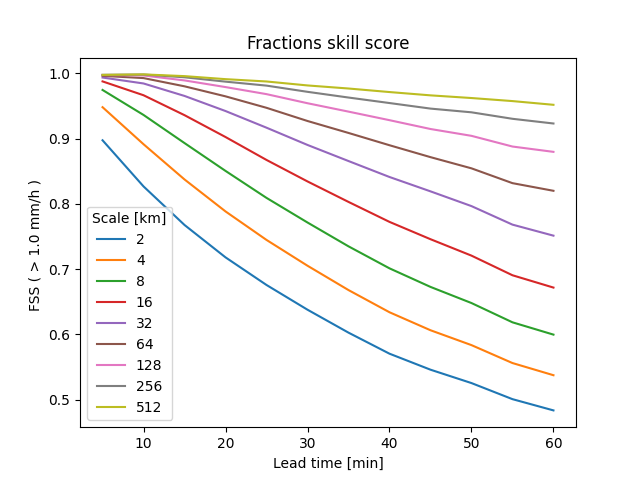
Verify with FSS#
The fractions skill score (FSS) provides an intuitive assessment of the dependency of skill on spatial scale and intensity, which makes it an ideal skill score for high-resolution precipitation forecasts.
# Find observations in the data archive
fns = io.archive.find_by_date(
    date,
    root_path,
    path_fmt,
    fn_pattern,
    fn_ext,
    timestep,
    num_prev_files=0,
    num_next_files=n_leadtimes,
)
# Read the radar composites
R_o, _, metadata_o = io.read_timeseries(fns, importer, **importer_kwargs)
R_o, metadata_o = conversion.to_rainrate(R_o, metadata_o, 223.0, 1.53)

# Compute fractions skill score (FSS) for all lead times, a set of scales and 1 mm/h
fss = verification.get_method("FSS")
scales = [2, 4, 8, 16, 32, 64, 128, 256, 512]
thr = 1.0
score = []
for i in range(n_leadtimes):
    score_ = []
    for scale in scales:
        score_.append(fss(R_f[i, :, :], R_o[i + 1, :, :], thr, scale))
    score.append(score_)

plt.figure()
x = np.arange(1, n_leadtimes + 1) * timestep
plt.plot(x, score)
plt.legend(scales, title="Scale [km]")
plt.xlabel("Lead time [min]")
plt.ylabel("FSS ( > 1.0 mm/h ) ")
plt.title("Fractions skill score")
plt.show()

# sphinx_gallery_thumbnail_number = 3
Total running time of the script: (0 minutes 7.345 seconds)