Note
Go to the end to download the full example code.
Optical flow#
This tutorial offers a short overview of the optical flow routines available in pysteps and it will cover how to compute and plot the motion field from a sequence of radar images.
from datetime import datetime
from pprint import pprint
import matplotlib.pyplot as plt
import numpy as np

from pysteps import io, motion, rcparams
from pysteps.utils import conversion, transformation
from pysteps.visualization import plot_precip_field, quiver
Read the radar input images#
First, we will import the sequence of radar composites. You need the pysteps-data archive downloaded and the pystepsrc file configured with the data_source paths pointing to data folders.
# Selected case
date = datetime.strptime("201505151630", "%Y%m%d%H%M")
data_source = rcparams.data_sources["mch"]
Load the data from the archive#
root_path = data_source["root_path"]
path_fmt = data_source["path_fmt"]
fn_pattern = data_source["fn_pattern"]
fn_ext = data_source["fn_ext"]
importer_name = data_source["importer"]
importer_kwargs = data_source["importer_kwargs"]
timestep = data_source["timestep"]

# Find the input files from the archive
fns = io.archive.find_by_date(
    date, root_path, path_fmt, fn_pattern, fn_ext, timestep=5, num_prev_files=9
)

# Read the radar composites
importer = io.get_method(importer_name, "importer")
R, quality, metadata = io.read_timeseries(fns, importer, **importer_kwargs)

del quality  # Not used
Preprocess the data#
# Convert to mm/h
R, metadata = conversion.to_rainrate(R, metadata)

# Store the reference frame
R_ = R[-1, :, :].copy()

# Log-transform the data [dBR]
R, metadata = transformation.dB_transform(R, metadata, threshold=0.1, zerovalue=-15.0)

# Nicely print the metadata
pprint(metadata)
{'accutime': 5,
 'cartesian_unit': 'm',
 'institution': 'MeteoSwiss',
 'product': 'AQC',
 'projection': '+proj=somerc  +lon_0=7.43958333333333 +lat_0=46.9524055555556 '
               '+k_0=1 +x_0=600000 +y_0=200000 +ellps=bessel '
               '+towgs84=674.374,15.056,405.346,0,0,0,0 +units=m +no_defs',
 'threshold': -10.0,
 'timestamps': array([datetime.datetime(2015, 5, 15, 15, 45),
       datetime.datetime(2015, 5, 15, 15, 50),
       datetime.datetime(2015, 5, 15, 15, 55),
       datetime.datetime(2015, 5, 15, 16, 0),
       datetime.datetime(2015, 5, 15, 16, 5),
       datetime.datetime(2015, 5, 15, 16, 10),
       datetime.datetime(2015, 5, 15, 16, 15),
       datetime.datetime(2015, 5, 15, 16, 20),
       datetime.datetime(2015, 5, 15, 16, 25),
       datetime.datetime(2015, 5, 15, 16, 30)], dtype=object),
 'transform': 'dB',
 'unit': 'mm/h',
 'x1': 255000.0,
 'x2': 965000.0,
 'xpixelsize': 1000.0,
 'y1': -160000.0,
 'y2': 480000.0,
 'yorigin': 'upper',
 'ypixelsize': 1000.0,
 'zerovalue': -15.0,
 'zr_a': 316.0,
 'zr_b': 1.5}
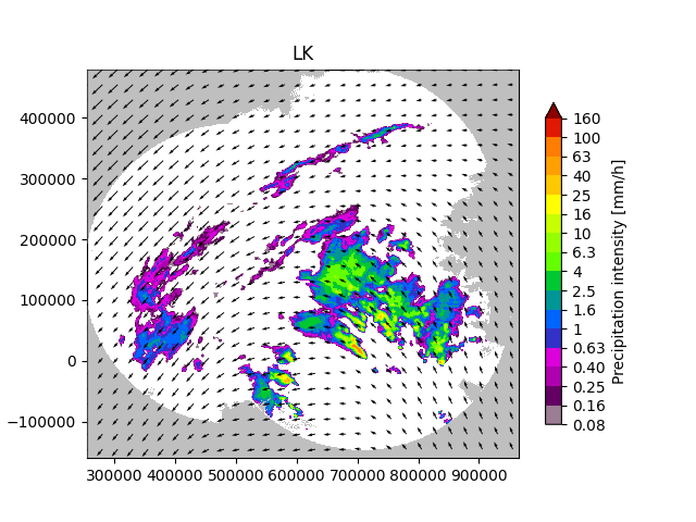
Lucas-Kanade (LK)#
The Lucas-Kanade optical flow method implemented in pysteps is a local tracking approach that relies on the OpenCV package. Local features are tracked in a sequence of two or more radar images. The scheme includes a final interpolation step in order to produce a smooth field of motion vectors.
oflow_method = motion.get_method("LK")
V1 = oflow_method(R[-3:, :, :])

# Plot the motion field on top of the reference frame
plot_precip_field(R_, geodata=metadata, title="LK")
quiver(V1, geodata=metadata, step=25)
plt.show()
/home/docs/checkouts/readthedocs.org/user_builds/pysteps/envs/stable/lib/python3.11/site-packages/pysteps/visualization/utils.py:439: UserWarning: cartopy package is required for the get_geogrid function but it is not installed. Ignoring geographical information.
  warnings.warn(
/home/docs/checkouts/readthedocs.org/user_builds/pysteps/envs/stable/lib/python3.11/site-packages/pysteps/visualization/utils.py:439: UserWarning: cartopy package is required for the get_geogrid function but it is not installed. Ignoring geographical information.
  warnings.warn(
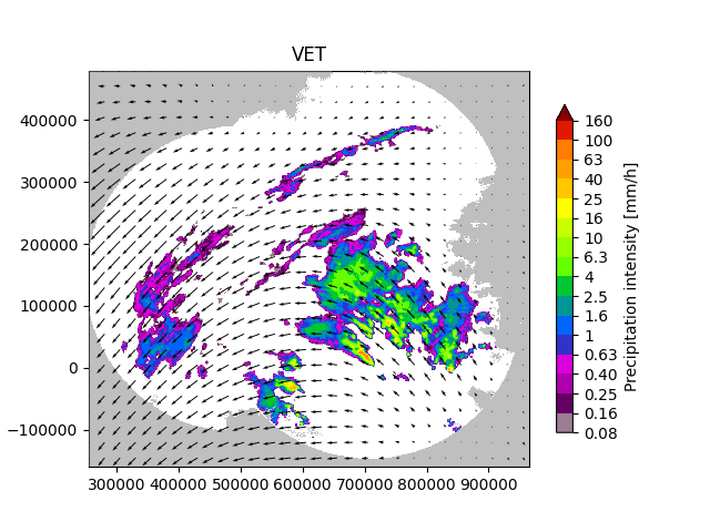
Variational echo tracking (VET)#
This module implements the VET algorithm presented by Laroche and Zawadzki (1995) and used in the McGill Algorithm for Prediction by Lagrangian Extrapolation (MAPLE) described in Germann and Zawadzki (2002). The approach essentially consists of a global optimization routine that seeks at minimizing a cost function between the displaced and the reference image.
oflow_method = motion.get_method("VET")
V2 = oflow_method(R[-3:, :, :])

# Plot the motion field
plot_precip_field(R_, geodata=metadata, title="VET")
quiver(V2, geodata=metadata, step=25)
plt.show()
Running VET algorithm
original image shape: (3, 640, 710)
padded image shape: (3, 640, 710)
padded template_image image shape: (3, 640, 710)

Number of sectors: 2,2
Sector Shape: (320, 355)
Minimizing

residuals 3102581.0581715787
smoothness_penalty 0.0
original image shape: (3, 640, 710)
padded image shape: (3, 640, 712)
padded template_image image shape: (3, 640, 712)

Number of sectors: 4,4
Sector Shape: (160, 178)
Minimizing

residuals 2508084.1906115236
smoothness_penalty 0.5085339537328549
original image shape: (3, 640, 710)
padded image shape: (3, 640, 720)
padded template_image image shape: (3, 640, 720)

Number of sectors: 16,16
Sector Shape: (40, 45)
Minimizing

residuals 2261616.6948113954
smoothness_penalty 38.22456746625133
original image shape: (3, 640, 710)
padded image shape: (3, 640, 736)
padded template_image image shape: (3, 640, 736)

Number of sectors: 32,32
Sector Shape: (20, 23)
Minimizing

residuals 2283382.409004245
smoothness_penalty 185.20525754821082
/home/docs/checkouts/readthedocs.org/user_builds/pysteps/envs/stable/lib/python3.11/site-packages/pysteps/visualization/utils.py:439: UserWarning: cartopy package is required for the get_geogrid function but it is not installed. Ignoring geographical information.
  warnings.warn(
/home/docs/checkouts/readthedocs.org/user_builds/pysteps/envs/stable/lib/python3.11/site-packages/pysteps/visualization/utils.py:439: UserWarning: cartopy package is required for the get_geogrid function but it is not installed. Ignoring geographical information.
  warnings.warn(
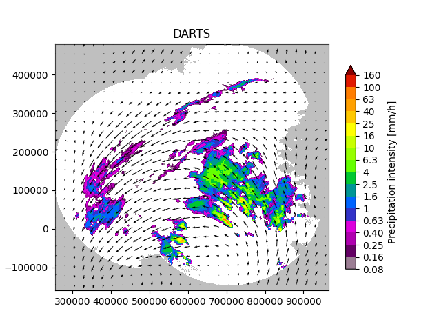
Dynamic and adaptive radar tracking of storms (DARTS)#
DARTS uses a spectral approach to optical flow that is based on the discrete Fourier transform (DFT) of a temporal sequence of radar fields. The level of truncation of the DFT coefficients controls the degree of smoothness of the estimated motion field, allowing for an efficient motion estimation. DARTS requires a longer sequence of radar fields for estimating the motion, here we are going to use all the available 10 fields.
oflow_method = motion.get_method("DARTS")
R[~np.isfinite(R)] = metadata["zerovalue"]
V3 = oflow_method(R)  # needs longer training sequence

# Plot the motion field
plot_precip_field(R_, geodata=metadata, title="DARTS")
quiver(V3, geodata=metadata, step=25)
plt.show()
Computing the motion field with the DARTS method.
-----
DARTS
-----
  Computing the FFT of the reflectivity fields...Done in 0.12 seconds.
  Constructing the y-vector...Done in 0.06 seconds.
  Constructing the H-matrix...Done in 0.93 seconds.
  Solving the linear systems...Done in 0.08 seconds.
--- 1.2247405052185059 seconds ---
/home/docs/checkouts/readthedocs.org/user_builds/pysteps/envs/stable/lib/python3.11/site-packages/pysteps/visualization/utils.py:439: UserWarning: cartopy package is required for the get_geogrid function but it is not installed. Ignoring geographical information.
  warnings.warn(
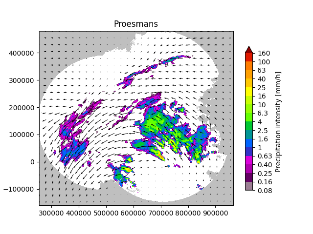
Anisotropic diffusion method (Proesmans et al 1994)#
This module implements the anisotropic diffusion method presented in Proesmans et al. (1994), a robust optical flow technique which employs the notion of inconsistency during the solution of the optical flow equations.
oflow_method = motion.get_method("proesmans")
R[~np.isfinite(R)] = metadata["zerovalue"]
V4 = oflow_method(R[-2:, :, :])

# Plot the motion field
plot_precip_field(R_, geodata=metadata, title="Proesmans")
quiver(V4, geodata=metadata, step=25)
plt.show()
/home/docs/checkouts/readthedocs.org/user_builds/pysteps/envs/stable/lib/python3.11/site-packages/pysteps/visualization/utils.py:439: UserWarning: cartopy package is required for the get_geogrid function but it is not installed. Ignoring geographical information.
  warnings.warn(
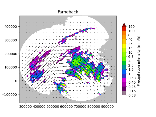
Farnebäck smoothed method#
This module implements the pyramidal decomposition method for motion estimation of Farnebäck as implemented in OpenCV, with an option for smoothing and renormalization of the motion fields proposed by Driedger et al.: https://cmosarchives.ca/Congress_P_A/program_abstracts2022.pdf (p. 392).
oflow_method = motion.get_method("farneback")
R[~np.isfinite(R)] = metadata["zerovalue"]
V5 = oflow_method(R[-2:, :, :], verbose=True)

# Plot the motion field
plot_precip_field(R_, geodata=metadata, title="Farneback")
quiver(V5, geodata=metadata, step=25)
plt.show()

# sphinx_gallery_thumbnail_number = 1
Computing the motion field with the Farneback method.
mult factor of smoothed motion field= 1.784774619115143
--- 0.44108080863952637 seconds ---
/home/docs/checkouts/readthedocs.org/user_builds/pysteps/envs/stable/lib/python3.11/site-packages/pysteps/visualization/utils.py:439: UserWarning: cartopy package is required for the get_geogrid function but it is not installed. Ignoring geographical information.
  warnings.warn(
Total running time of the script: (0 minutes 35.826 seconds)