Generation of stochastic noise

This example script shows how to run the stochastic noise field generators included in pysteps.

These noise fields are used as perturbation terms during an extrapolation nowcast in order to represent the uncertainty in the evolution of the rainfall field.

from matplotlib import cm, pyplot as plt
import numpy as np
import os
from pprint import pprint
from pysteps import io, rcparams
from pysteps.noise.fftgenerators import initialize_param_2d_fft_filter
from pysteps.noise.fftgenerators import initialize_nonparam_2d_fft_filter
from pysteps.noise.fftgenerators import generate_noise_2d_fft_filter
from pysteps.utils import conversion, rapsd, transformation
from pysteps.visualization import plot_precip_field, plot_spectrum1d

Read precipitation field

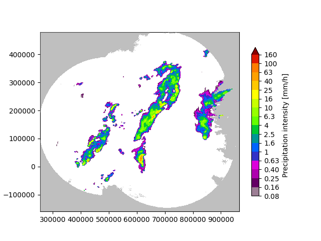
First thing, the radar composite is imported and transformed in units of dB. This image will be used to train the Fourier filters that are necessary to produce the fields of spatially correlated noise.

# Import the example radar composite
root_path = rcparams.data_sources["mch"]["root_path"]
filename = os.path.join(root_path, "20160711", "AQC161932100V_00005.801.gif")
R, _, metadata = io.import_mch_gif(filename, product="AQC", unit="mm", accutime=5.0)

# Convert to mm/h
R, metadata = conversion.to_rainrate(R, metadata)

# Nicely print the metadata
pprint(metadata)

# Plot the rainfall field
plot_precip_field(R, geodata=metadata)
plt.show()

# Log-transform the data
R, metadata = transformation.dB_transform(R, metadata, threshold=0.1, zerovalue=-15.0)

# Assign the fill value to all the Nans
R[~np.isfinite(R)] = metadata["zerovalue"]

{'accutime': 5.0,
 'cartesian_unit': 'm',
 'institution': 'MeteoSwiss',
 'product': 'AQC',
 'projection': '+proj=somerc  +lon_0=7.43958333333333 +lat_0=46.9524055555556 '
               '+k_0=1 +x_0=600000 +y_0=200000 +ellps=bessel '
               '+towgs84=674.374,15.056,405.346,0,0,0,0 +units=m +no_defs',
 'threshold': 0.01155375598376629,
 'transform': None,
 'unit': 'mm/h',
 'x1': 255000.0,
 'x2': 965000.0,
 'xpixelsize': 1000.0,
 'y1': -160000.0,
 'y2': 480000.0,
 'yorigin': 'upper',
 'ypixelsize': 1000.0,
 'zerovalue': 0.0,
 'zr_a': 316.0,
 'zr_b': 1.5}
/home/docs/checkouts/readthedocs.org/user_builds/pysteps/envs/stable/lib/python3.10/site-packages/pysteps/visualization/utils.py:439: UserWarning: cartopy package is required for the get_geogrid function but it is not installed. Ignoring geographical information.
  warnings.warn(

Parametric filter

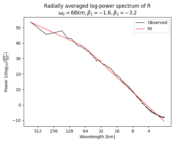
In the parametric approach, a power-law model is used to approximate the power spectral density (PSD) of a given rainfall field.

The parametric model uses a piece-wise linear function with two spectral slopes (beta1 and beta2) and one breaking point

# Fit the parametric PSD to the observation
Fp = initialize_param_2d_fft_filter(R)

# Compute the observed and fitted 1D PSD
L = np.max(Fp["input_shape"])
if L % 2 == 1:
    wn = np.arange(0, int(L / 2) + 1)
else:
    wn = np.arange(0, int(L / 2))
R_, freq = rapsd(R, fft_method=np.fft, return_freq=True)
f = np.exp(Fp["model"](np.log(wn), *Fp["pars"]))

# Extract the scaling break in km, beta1 and beta2
w0 = L / np.exp(Fp["pars"][0])
b1 = Fp["pars"][2]
b2 = Fp["pars"][3]

# Plot the observed power spectrum and the model
fig, ax = plt.subplots()
plot_scales = [512, 256, 128, 64, 32, 16, 8, 4]
plot_spectrum1d(
    freq,
    R_,
    x_units="km",
    y_units="dBR",
    color="k",
    ax=ax,
    label="Observed",
    wavelength_ticks=plot_scales,
)
plot_spectrum1d(
    freq,
    f,
    x_units="km",
    y_units="dBR",
    color="r",
    ax=ax,
    label="Fit",
    wavelength_ticks=plot_scales,
)
plt.legend()
ax.set_title(
    "Radially averaged log-power spectrum of R\n"
    r"$\omega_0=%.0f km, \beta_1=%.1f, \beta_2=%.1f$" % (w0, b1, b2)
)
plt.show()

Nonparametric filter

In the nonparametric approach, the Fourier filter is obtained directly from the power spectrum of the observed precipitation field R.

Fnp = initialize_nonparam_2d_fft_filter(R)

Noise generator

The parametric and nonparametric filters obtained above can now be used to produce N realizations of random fields of prescribed power spectrum, hence with the same correlation structure as the initial rainfall field.

seed = 42
num_realizations = 3

# Generate noise
Np = []
Nnp = []
for k in range(num_realizations):
    Np.append(generate_noise_2d_fft_filter(Fp, seed=seed + k))
    Nnp.append(generate_noise_2d_fft_filter(Fnp, seed=seed + k))

# Plot the generated noise fields

fig, ax = plt.subplots(nrows=2, ncols=3)

# parametric noise
ax[0, 0].imshow(Np[0], cmap=cm.RdBu_r, vmin=-3, vmax=3)
ax[0, 1].imshow(Np[1], cmap=cm.RdBu_r, vmin=-3, vmax=3)
ax[0, 2].imshow(Np[2], cmap=cm.RdBu_r, vmin=-3, vmax=3)

# nonparametric noise
ax[1, 0].imshow(Nnp[0], cmap=cm.RdBu_r, vmin=-3, vmax=3)
ax[1, 1].imshow(Nnp[1], cmap=cm.RdBu_r, vmin=-3, vmax=3)
ax[1, 2].imshow(Nnp[2], cmap=cm.RdBu_r, vmin=-3, vmax=3)

for i in range(2):
    for j in range(3):
        ax[i, j].set_xticks([])
        ax[i, j].set_yticks([])
plt.tight_layout()
plt.show()

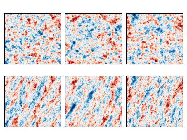
The above figure highlights the main limitation of the parametric approach (top row), that is, the assumption of an isotropic power law scaling relationship, meaning that anisotropic structures such as rainfall bands cannot be represented.

Instead, the nonparametric approach (bottom row) allows generating perturbation fields with anisotropic structures, but it also requires a larger sample size and is sensitive to the quality of the input data, e.g. the presence of residual clutter in the radar image.

In addition, both techniques assume spatial stationarity of the covariance structure of the field.

# sphinx_gallery_thumbnail_number = 3