Ensemble-based Blending

This tutorial demonstrates how to construct a blended rainfall forecast by combining an ensemble nowcast with an ensemble Numerical Weather Prediction (NWP) forecast. The method follows the Reduced-Space Ensemble Kalman Filter approach described in [NFL+19].

The procedure starts from the most recent radar observations. In the prediction step, a stochastic radar extrapolation technique generates short-term forecasts. In the correction step, these forecasts are updated using information from the latest ensemble NWP run. To make the matrix operations tractable, the Bayesian update is carried out in the subspace defined by the leading principal components—hence the term reduced space.

The datasets used in this tutorial are provided by the German Weather Service (DWD).

import os
from datetime import datetime, timedelta

import numpy as np
from matplotlib import pyplot as plt

import pysteps
from pysteps import io, rcparams, blending
from pysteps.utils import aggregate_fields_space
from pysteps.visualization import plot_precip_field
import pysteps_nwp_importers

Read the radar images and the NWP forecast

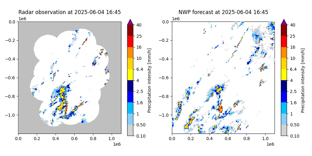
First, we import a sequence of 4 images of 5-minute radar composites and the corresponding NWP rainfall forecast that was available at that time.

You need the pysteps-data archive downloaded and the pystepsrc file configured with the data_source paths pointing to data folders. Additionally, the pysteps-nwp-importers plugin needs to be installed, see pySTEPS/pysteps-nwp-importers.

# Selected case
date_radar = datetime.strptime("202506041645", "%Y%m%d%H%M")
# The last NWP forecast was issued at 16:00 - the blending tool will be able
# to find the correct lead times itself.
date_nwp = datetime.strptime("202506041600", "%Y%m%d%H%M")
radar_data_source = rcparams.data_sources["dwd"]
nwp_data_source = rcparams.data_sources["dwd_nwp"]

Load the data from the archive

root_path = radar_data_source["root_path"]
path_fmt = radar_data_source["path_fmt"]
fn_pattern = radar_data_source["fn_pattern"]
fn_ext = radar_data_source["fn_ext"]
importer_name = radar_data_source["importer"]
importer_kwargs = radar_data_source["importer_kwargs"]
timestep_radar = radar_data_source["timestep"]

# Find the radar files in the archive
fns = io.find_by_date(
    date_radar,
    root_path,
    path_fmt,
    fn_pattern,
    fn_ext,
    timestep_radar,
    num_prev_files=2,
)

# Read the radar composites (which are already in mm/h)
importer = io.get_method(importer_name, "importer")
radar_precip, _, radar_metadata = io.read_timeseries(fns, importer, **importer_kwargs)

# Import the NWP data
filename = os.path.join(
    nwp_data_source["root_path"],
    datetime.strftime(date_nwp, nwp_data_source["path_fmt"]),
    datetime.strftime(date_nwp, nwp_data_source["fn_pattern"])
    + "."
    + nwp_data_source["fn_ext"],
)
nwp_importer = io.get_method("dwd_nwp", "importer")
kwargs = nwp_data_source["importer_kwargs"]
# Resolve grid_file_path relative to PYSTEPS_DATA_PATH
kwargs["grid_file_path"] = os.path.join(
    os.environ["PYSTEPS_DATA_PATH"], kwargs["grid_file_path"]
)
nwp_precip, _, nwp_metadata = nwp_importer(filename, **kwargs)
# We lower the number of ens members to 10 to reduce the memory needs in the
# example here. However, it is advised to have a minimum of 20 members for the
# Reduced-Space Ensemble Kalman filter approach
nwp_precip = nwp_precip[:, 0:10, :].astype("single")

Pre-processing steps

# Set the zerovalue and precipitation thresholds (these are fixed from DWD)
prec_thr = 0.049
zerovalue = 0.027

# Transform the zerovalue and precipitation thresholds to dBR
log_thr_prec = 10.0 * np.log10(prec_thr)
log_zerovalue = 10.0 * np.log10(zerovalue)

# Reproject the DWD ICON NWP data onto a regular grid
nwp_metadata["clon"] = nwp_precip["longitude"].values
nwp_metadata["clat"] = nwp_precip["latitude"].values
# We change the time step from the DWD NWP data to 15 min (it is actually 5 min)
# to have a longer forecast horizon available for this example, as pysteps_data
# only contains 1 hour of DWD forecast data (to minimize storage).
nwp_metadata["accutime"] = 15.0
nwp_precip = (
    nwp_precip.values.astype("single") * 3.0
)  # (to account for the change in time step from 5 to 15 min)

# Reproject ID2 data onto a regular grid
nwp_precip_rprj, nwp_metadata_rprj = (
    pysteps_nwp_importers.importer_dwd_nwp.unstructured2regular(
        nwp_precip, nwp_metadata, radar_metadata
    )
)
nwp_precip = None

# Upscale both the radar and NWP data to a twice as coarse resolution to lower
# the memory needs (for this example)
radar_precip, radar_metadata = aggregate_fields_space(
    radar_precip, radar_metadata, radar_metadata["xpixelsize"] * 4
)
nwp_precip_rprj, nwp_metadata_rprj = aggregate_fields_space(
    nwp_precip_rprj.astype("single"),
    nwp_metadata_rprj,
    nwp_metadata_rprj["xpixelsize"] * 4,
)

# Make sure the units are in mm/h
converter = pysteps.utils.get_method("mm/h")
radar_precip, radar_metadata = converter(
    radar_precip, radar_metadata
)  # The radar data should already be in mm/h
nwp_precip_rprj, nwp_metadata_rprj = converter(nwp_precip_rprj, nwp_metadata_rprj)

# Threshold the data
radar_precip[radar_precip < prec_thr] = 0.0
nwp_precip_rprj[nwp_precip_rprj < prec_thr] = 0.0

# Plot the radar rainfall field and the first time step and first ensemble member
# of the NWP forecast.
date_str = datetime.strftime(date_radar, "%Y-%m-%d %H:%M")
plt.figure(figsize=(10, 5))
plt.subplot(121)
plot_precip_field(
    radar_precip[-1, :, :],
    geodata=radar_metadata,
    title=f"Radar observation at {date_str}",
    colorscale="STEPS-NL",
)
plt.subplot(122)
plot_precip_field(
    nwp_precip_rprj[0, 0, :, :],
    geodata=nwp_metadata_rprj,
    title=f"NWP forecast at {date_str}",
    colorscale="STEPS-NL",
)
plt.tight_layout()
plt.show()

# transform the data to dB
transformer = pysteps.utils.get_method("dB")
radar_precip, radar_metadata = transformer(
    radar_precip, radar_metadata, threshold=prec_thr, zerovalue=log_zerovalue
)
nwp_precip_rprj, nwp_metadata_rprj = transformer(
    nwp_precip_rprj, nwp_metadata_rprj, threshold=prec_thr, zerovalue=log_zerovalue
)

Determine the velocity fields

In contrast to the STEPS blending method, no motion field for the NWP fields is needed in the ensemble kalman filter blending approach.

# Estimate the motion vector field
oflow_method = pysteps.motion.get_method("lucaskanade")
velocity_radar = oflow_method(radar_precip)

The blended forecast

# Set the timestamps for radar_precip and nwp_precip_rprj
timestamps_radar = np.array(
    sorted(
        [
            date_radar - timedelta(minutes=i * timestep_radar)
            for i in range(len(radar_precip))
        ]
    )
)
timestamps_nwp = np.array(
    sorted(
        [
            date_nwp + timedelta(minutes=i * int(nwp_metadata_rprj["accutime"]))
            for i in range(nwp_precip_rprj.shape[0])
        ]
    )
)

# Set the combination kwargs
combination_kwargs = dict(
    n_tapering=0,  # Tapering parameter: controls how many diagonals of the covariance matrix are kept (0 = no tapering)
    non_precip_mask=True,  # Specifies whether the computation should be truncated on grid boxes where at least a minimum number of ens. members forecast precipitation.
    n_ens_prec=1,  # Minimum number of ens. members that forecast precip for the above-mentioned mask.
    lien_criterion=True,  # Specifies wheter the Lien criterion should be applied.
    n_lien=5,  # Minimum number of ensemble members that forecast precipitation for the Lien criterion (equals half the ens. members here)
    prob_matching="iterative",  # The type of probability matching used.
    inflation_factor_bg=3.0,  # Inflation factor of the background (NWC) covariance matrix. (this value indicates a faster convergence towards the NWP ensemble)
    inflation_factor_obs=1.0,  # Inflation factor of the observation (NWP) covariance matrix.
    offset_bg=0.0,  # Offset of the background (NWC) covariance matrix.
    offset_obs=0.0,  # Offset of the observation (NWP) covariance matrix.
    nwp_hres_eff=14.0,  # Effective horizontal resolution of the utilized NWP model (in km here).
    sampling_prob_source="ensemble",  # Computation method of the sampling probability for the probability matching. 'ensemble' computes this probability as the ratio between the ensemble differences.
    use_accum_sampling_prob=False,  # Specifies whether the current sampling probability should be used for the probability matching or a probability integrated over the previous forecast time.
)


# Call the PCA EnKF method
blending_method = blending.get_method("pca_enkf")
precip_forecast = blending_method(
    obs_precip=radar_precip,  # Radar data in dBR
    obs_timestamps=timestamps_radar,  # Radar timestamps
    nwp_precip=nwp_precip_rprj,  # NWP in dBR
    nwp_timestamps=timestamps_nwp,  # NWP timestamps
    velocity=velocity_radar,  # Velocity vector field
    forecast_horizon=120,  # Forecast length (horizon) in minutes - only a short forecast horizon due to the limited dataset length stored here.
    issuetime=date_radar,  # Forecast issue time as datetime object
    n_ens_members=10,  # No. of ensemble members
    precip_mask_dilation=1,  # Dilation of precipitation mask in grid boxes
    n_cascade_levels=6,  # No. of cascade levels
    precip_thr=log_thr_prec,  # Precip threshold
    norain_thr=0.0005,  # Minimum of 0.5% precip needed, otherwise 'zero rainfall'
    num_workers=4,  # No. of parallel threads
    noise_stddev_adj="auto",  # Standard deviation adjustment
    noise_method="ssft",  # SSFT as noise method
    enable_combination=True,  # Enable combination
    noise_kwargs={"win_size": (512, 512), "win_fun": "hann", "overlap": 0.5},
    extrap_kwargs={"interp_order": 3, "map_coordinates_mode": "nearest"},
    combination_kwargs=combination_kwargs,
    filter_kwargs={"include_mean": True},
)

# Transform the data back into mm/h
precip_forecast, _ = converter(precip_forecast, radar_metadata)
radar_precip, _ = converter(radar_precip, radar_metadata)
nwp_precip, _ = converter(nwp_precip_rprj, nwp_metadata_rprj)

Test for no rain cases
======================

Rain fraction is: 0.08794545454545455, while minimum fraction is 0.0005
Rain fraction is: 0.14362814814814814, while minimum fraction is 0.0005
Reduced-space ensemble Kalman filter
====================================

Inputs
------
Forecast issue time:                2025-06-04T16:45:00
Input dimensions:                   300x275
Temporal resolution:                5 minutes

NWP and blending inputs
-----------------------
Number of (NWP) models:             10

Methods
-------
Extrapolation:                      semilagrangian
Bandpass filter:                    gaussian
Decomposition:                      fft
Noise generator:                    ssft
Noise adjustment:                   yes
EnKF implementation:                masked_enkf
FFT method:                         numpy
Domain:                             spatial

Parameters
----------
Forecast length in min:             120
Ensemble size:                      10
Parallel threads:                   4
Number of cascade levels:           6
Order of the AR(p) model:           1

No rain forecast:                   none
Nowcast components initialized successfully.
************************************************
* Correlation coefficients for cascade levels: *
************************************************
-------------------------
| Level |     Lag-1     |
-------------------------
| 1     | 0.999399      |
-------------------------
| 2     | 0.996212      |
-------------------------
| 3     | 0.988787      |
-------------------------
| 4     | 0.972267      |
-------------------------
| 5     | 0.904330      |
-------------------------
| 6     | 0.578820      |
-------------------------
****************************************
* AR(p) parameters for cascade levels: *
****************************************
---------------------------------------
| Level |    Phi-1     |    Phi-0     |
---------------------------------------
| 1     | 0.999399     | 0.034674     |
---------------------------------------
| 2     | 0.996212     | 0.086954     |
---------------------------------------
| 3     | 0.988787     | 0.149329     |
---------------------------------------
| 4     | 0.972267     | 0.233874     |
---------------------------------------
| 5     | 0.904330     | 0.426835     |
---------------------------------------
| 6     | 0.578820     | 0.815456     |
---------------------------------------
Computing noise adjustment coefficients... noise std. dev. coeffs:   [1.20439368 1.16941322 1.01525735 1.11890008 1.05759501 0.74970358]
Initialize ensemble Kalman filter
=================================

Non-tapered diagonals:              0
Non precip mask:                    True
No. ens mems with precipitation:    1
Lien Criterion:                     True
No. ens mems with precip (Lien):    5

Initialize masked ensemble Kalman filter
========================================

Iterative probability matching:     True
Background inflation factor:        3.0
Observation inflation factor:       1.0
Background offset:                  0.0
Observation offset:                 0.0
Sampling probability source:        ensemble
Use accum. sampling probability:    False
Ensure full NWP weight:             True
Computing combination for lead time + 0 min
...done.
Computing combination for lead time + 5 min
...done.
Computing combination for lead time + 10 min
...done.
Computing combination for lead time + 15 min
...done.
Computing combination for lead time + 20 min
Sampling probability: 0.0396
...done.
Computing combination for lead time + 25 min
...done.
Computing combination for lead time + 30 min
...done.
Computing combination for lead time + 35 min
Sampling probability: 0.0573
...done.
Computing combination for lead time + 40 min
...done.
Computing combination for lead time + 45 min
...done.
Computing combination for lead time + 50 min
Sampling probability: 0.1833
...done.
Computing combination for lead time + 55 min
...done.
Computing combination for lead time + 60 min
...done.
Computing combination for lead time + 65 min
Sampling probability: 0.8115
...done.
Computing combination for lead time + 70 min
...done.
Computing combination for lead time + 75 min
...done.
Computing combination for lead time + 80 min
Sampling probability: 0.5703
...done.
Computing combination for lead time + 85 min
...done.
Computing combination for lead time + 90 min
...done.
Computing combination for lead time + 95 min
Sampling probability: 0.8174
...done.
Computing combination for lead time + 100 min
...done.
Computing combination for lead time + 105 min
...done.
Computing combination for lead time + 110 min
Sampling probability: 0.8645
...done.
Computing combination for lead time + 115 min
...done.
Computing combination for lead time + 120 min
...done.

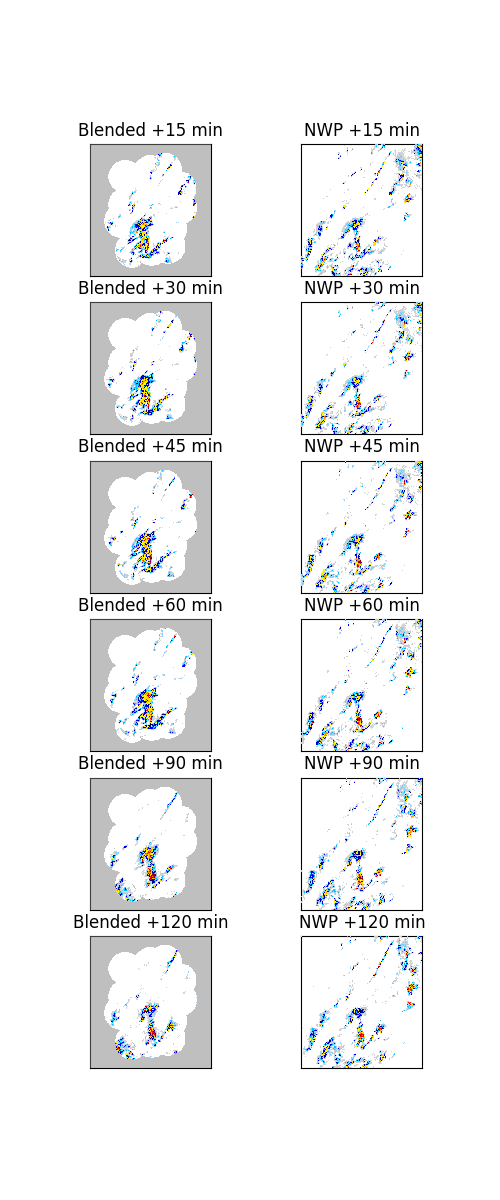
Visualize the output

The NWP rainfall forecast has a much lower weight than the radar-based extrapolation # forecast at the issue time of the forecast (+0 min). Therefore, the first time steps consist mostly of the extrapolation. However, near the end of the forecast (+180 min), the NWP share in the blended forecast has become the more dominant contribution to the forecast and thus the forecast starts to resemble the NWP forecast.

fig = plt.figure(figsize=(5, 12))

leadtimes_min = [15, 30, 45, 60, 90, 120]
n_leadtimes = len(leadtimes_min)
for n, leadtime in enumerate(leadtimes_min):
    # Nowcast with blending into NWP
    plt.subplot(n_leadtimes, 2, n * 2 + 1)
    plot_precip_field(
        precip_forecast[0, int(leadtime / timestep_radar) - 1, :, :],
        geodata=radar_metadata,
        title=f"Blended +{leadtime} min",
        axis="off",
        colorscale="STEPS-NL",
        colorbar=False,
    )

    # Raw NWP forecast
    plt.subplot(n_leadtimes, 2, n * 2 + 2)
    plot_precip_field(
        nwp_precip[int(leadtime / int(nwp_metadata_rprj["accutime"])) - 1, 0, :, :],
        geodata=nwp_metadata_rprj,
        title=f"NWP +{leadtime} min",
        axis="off",
        colorscale="STEPS-NL",
        colorbar=False,
    )

References

# Nerini, D., Foresti, L., Leuenberger, D., Robert, S., Germann, U. 2019. "A
# Reduced-Space Ensemble Kalman Filter Approach for Flow-Dependent Integration
# of Radar Extrapolation Nowcasts and NWP Precipitation Ensembles." Monthly
# Weather Review 147(3): 987-1006. https://doi.org/10.1175/MWR-D-18-0258.1.