Optical flow

This tutorial offers a short overview of the optical flow routines available in pysteps and it will cover how to compute and plot the motion field from a sequence of radar images.

from datetime import datetime
import numpy as np
from pprint import pprint
from pysteps import io, motion, rcparams
from pysteps.utils import conversion, transformation
from pysteps.visualization import plot_precip_field, quiver

Read the radar input images

First thing, the sequence of radar composites is imported, converted and transformed into units of dBR.

date = datetime.strptime("201505151630", "%Y%m%d%H%M")
data_source = "mch"

# Load data source config
root_path = rcparams.data_sources[data_source]["root_path"]
path_fmt = rcparams.data_sources[data_source]["path_fmt"]
fn_pattern = rcparams.data_sources[data_source]["fn_pattern"]
fn_ext = rcparams.data_sources[data_source]["fn_ext"]
importer_name = rcparams.data_sources[data_source]["importer"]
importer_kwargs = rcparams.data_sources[data_source]["importer_kwargs"]
timestep = rcparams.data_sources[data_source]["timestep"]

# Find the input files from the archive
fns = io.archive.find_by_date(
    date, root_path, path_fmt, fn_pattern, fn_ext, timestep, num_prev_files=9
)

# Read the radar composites
importer = io.get_method(importer_name, "importer")
R, _, metadata = io.read_timeseries(fns, importer, **importer_kwargs)

# Convert to mm/h
R, metadata = conversion.to_rainrate(R, metadata)

# Store the last frame for polotting it later later
R_ = R[-1, :, :].copy()

# Log-transform the data
R, metadata = transformation.dB_transform(R, metadata, threshold=0.1, zerovalue=-15.0)

# Nicely print the metadata
pprint(metadata)

Out:

{'accutime': 5,
 'institution': 'MeteoSwiss',
 'product': 'AQC',
 'projection': '+proj=somerc  +lon_0=7.43958333333333 +lat_0=46.9524055555556 '
               '+k_0=1 +x_0=600000 +y_0=200000 +ellps=bessel '
               '+towgs84=674.374,15.056,405.346,0,0,0,0 +units=m +no_defs',
 'threshold': -10.0,
 'timestamps': array([datetime.datetime(2015, 5, 15, 15, 45),
       datetime.datetime(2015, 5, 15, 15, 50),
       datetime.datetime(2015, 5, 15, 15, 55),
       datetime.datetime(2015, 5, 15, 16, 0),
       datetime.datetime(2015, 5, 15, 16, 5),
       datetime.datetime(2015, 5, 15, 16, 10),
       datetime.datetime(2015, 5, 15, 16, 15),
       datetime.datetime(2015, 5, 15, 16, 20),
       datetime.datetime(2015, 5, 15, 16, 25),
       datetime.datetime(2015, 5, 15, 16, 30)], dtype=object),
 'transform': 'dB',
 'unit': 'mm/h',
 'x1': 255000.0,
 'x2': 965000.0,
 'xpixelsize': 1000.0,
 'y1': -160000.0,
 'y2': 480000.0,
 'yorigin': 'upper',
 'ypixelsize': 1000.0,
 'zerovalue': -15.0}

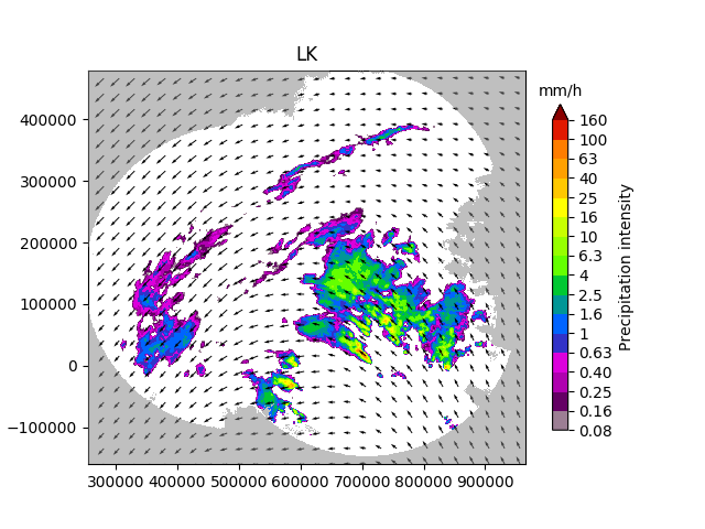
Lucas-Kanade (LK)

The Lucas-Kanade optical flow method implemented in pysteps is a local tracking approach that relies on the OpenCV package. Local features are tracked in a sequence of two or more radar images. The scheme includes a final interpolation step in order to produce a smooth field of motion vectors.

oflow_method = motion.get_method("LK")
V1 = oflow_method(R[-3:, :, :])

# Plot the motion field
plot_precip_field(R_, geodata=metadata, title="LK")
quiver(V1, geodata=metadata, step=25)

Out:

Computing the motion field with the Lucas-Kanade method.
--- LK found 392 sparse vectors ---
--- 158 sparse vectors left for interpolation ---
--- 1.11 seconds ---

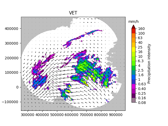
Variational echo tracking (VET)

This module implements the VET algorithm presented by Laroche and Zawadzki (1995) and used in the McGill Algorithm for Prediction by Lagrangian Extrapolation (MAPLE) described in Germann and Zawadzki (2002). The approach essentially consists of a global optimization routine that seeks at minimizing a cost function between the displaced and the reference image.

oflow_method = motion.get_method("VET")
V2 = oflow_method(R[-3:, :, :])

# Plot the motion field
plot_precip_field(R_, geodata=metadata, title="VET")
quiver(V2, geodata=metadata, step=25)

Out:

Running VET algorithm
original image shape: (3, 640, 710)
padded image shape: (3, 640, 710)
padded template_image image shape: (3, 640, 710)

Number of sectors: 2,2
Sector Shape: (320, 355)
Minimizing

residuals 3860502.2323758407
smoothness_penalty 0.0
original image shape: (3, 640, 712)
padded image shape: (3, 640, 712)
padded template_image image shape: (3, 640, 712)

Number of sectors: 4,4
Sector Shape: (160, 178)
Minimizing

residuals 2852728.474075019
smoothness_penalty 1.2934717610147382
original image shape: (3, 640, 720)
padded image shape: (3, 640, 720)
padded template_image image shape: (3, 640, 720)

Number of sectors: 16,16
Sector Shape: (40, 45)
Minimizing

residuals 2591853.9497765535
smoothness_penalty 98.75780333213032
original image shape: (3, 640, 736)
padded image shape: (3, 640, 736)
padded template_image image shape: (3, 640, 736)

Number of sectors: 32,32
Sector Shape: (20, 23)
Minimizing

residuals 2615161.846366342
smoothness_penalty 309.47364391248857

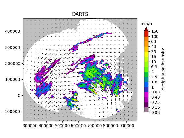
Dynamic and adaptive radar tracking of storms (DARTS)

DARTS uses a spectral approach to optical flow that is based on the discrete Fourier transform (DFT) of a temporal sequence of radar fields. The level of truncation of the DFT coefficients controls the degree of smoothness of the estimated motion field, allowing for an efficient motion estimation. DARTS requires a longer sequence of radar fields for estimating the motion, here we are going to use all the available 10 fields.

oflow_method = motion.get_method("DARTS")
R[~np.isfinite(R)] = metadata["zerovalue"]
V3 = oflow_method(R)  # needs longer training sequence

# Plot the motion field
plot_precip_field(R_, geodata=metadata, title="DARTS")
quiver(V3, geodata=metadata, step=25)

# sphinx_gallery_thumbnail_number = 1

Out:

Computing the motion field with the DARTS method.
--- 3.309852361679077 seconds ---