Ensemble verification

This tutorial shows how to compute and plot an extrapolation nowcast using Finnish radar data.

from pylab import *
from datetime import datetime
from pprint import pprint
from pysteps import io, nowcasts, rcparams, verification
from pysteps.motion.lucaskanade import dense_lucaskanade
from pysteps.postprocessing import ensemblestats
from pysteps.utils import conversion, dimension, transformation
from pysteps.visualization import plot_precip_field

# Set nowcast parameters
n_ens_members = 20
n_leadtimes = 6
seed = 24

Read precipitation field

First thing, the sequence of Swiss radar composites is imported, converted and transformed into units of dBR.

date = datetime.strptime("201607112100", "%Y%m%d%H%M")
data_source = "mch"

# Load data source config
root_path = rcparams.data_sources[data_source]["root_path"]
path_fmt = rcparams.data_sources[data_source]["path_fmt"]
fn_pattern = rcparams.data_sources[data_source]["fn_pattern"]
fn_ext = rcparams.data_sources[data_source]["fn_ext"]
importer_name = rcparams.data_sources[data_source]["importer"]
importer_kwargs = rcparams.data_sources[data_source]["importer_kwargs"]
timestep = rcparams.data_sources[data_source]["timestep"]

# Find the radar files in the archive
fns = io.find_by_date(
    date, root_path, path_fmt, fn_pattern, fn_ext, timestep, num_prev_files=2
)

# Read the data from the archive
importer = io.get_method(importer_name, "importer")
R, _, metadata = io.read_timeseries(fns, importer, **importer_kwargs)

# Convert to rain rate
R, metadata = conversion.to_rainrate(R, metadata)

# Upscale data to 2 km to limit memory usage
R, metadata = dimension.aggregate_fields_space(R, metadata, 2000)

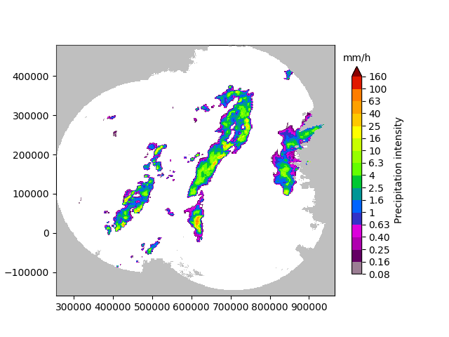
# Plot the rainfall field
plot_precip_field(R[-1, :, :], geodata=metadata)

# Log-transform the data to unit of dBR, set the threshold to 0.1 mm/h,
# set the fill value to -15 dBR
R, metadata = transformation.dB_transform(R, metadata, threshold=0.1, zerovalue=-15.0)

# Set missing values with the fill value
R[~np.isfinite(R)] = -15.0

# Nicely print the metadata
pprint(metadata)

Out:

{'accutime': 5,
 'institution': 'MeteoSwiss',
 'product': 'AQC',
 'projection': '+proj=somerc  +lon_0=7.43958333333333 +lat_0=46.9524055555556 '
               '+k_0=1 +x_0=600000 +y_0=200000 +ellps=bessel '
               '+towgs84=674.374,15.056,405.346,0,0,0,0 +units=m +no_defs',
 'threshold': -10.0,
 'timestamps': array([datetime.datetime(2016, 7, 11, 20, 50),
       datetime.datetime(2016, 7, 11, 20, 55),
       datetime.datetime(2016, 7, 11, 21, 0)], dtype=object),
 'transform': 'dB',
 'unit': 'mm/h',
 'x1': 255000.0,
 'x2': 965000.0,
 'xpixelsize': 2000,
 'y1': -160000.0,
 'y2': 480000.0,
 'yorigin': 'upper',
 'ypixelsize': 2000,
 'zerovalue': -15.0}

Forecast

We use the STEPS approach to produce a ensemble nowcast of precipitation fields.

# Estimate the motion field
V = dense_lucaskanade(R)

# The STEPES nowcast
nowcast_method = nowcasts.get_method("steps")
R_f = nowcast_method(
    R[-3:, :, :],
    V,
    n_leadtimes,
    n_ens_members,
    n_cascade_levels=6,
    R_thr=-10.0,
    kmperpixel=2.0,
    timestep=timestep,
    decomp_method="fft",
    bandpass_filter_method="gaussian",
    noise_method="nonparametric",
    vel_pert_method="bps",
    mask_method="incremental",
    seed=seed,
)

# Back-transform to rain rates
R_f = transformation.dB_transform(R_f, threshold=-10.0, inverse=True)[0]

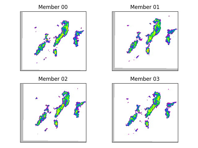
# Plot some of the realizations
fig = figure()
for i in range(4):
    ax = fig.add_subplot(221 + i)
    ax.set_title("Member %02d" % i)
    plot_precip_field(R_f[i, -1, :, :], geodata=metadata, colorbar=False, axis="off")
tight_layout()

Out:

Computing the motion field with the Lucas-Kanade method.
--- LK found 143 sparse vectors ---
--- 57 sparse vectors left for interpolation ---
--- 0.28 seconds ---
Computing STEPS nowcast:
------------------------

Inputs:
-------
input dimensions: 320x355
km/pixel:         2
time step:        5 minutes

Methods:
--------
extrapolation:          semilagrangian
bandpass filter:        gaussian
decomposition:          fft
noise generator:        nonparametric
noise adjustment:       no
velocity perturbator:   bps
conditional statistics: no
precip. mask method:    incremental
probability matching:   cdf
FFT method:             numpy

Parameters:
-----------
number of time steps:     6
ensemble size:            20
parallel threads:         1
number of cascade levels: 6
order of the AR(p) model: 2
velocity perturbations, parallel:      10.88,0.23,-7.68
velocity perturbations, perpendicular: 5.76,0.31,-2.72
precip. intensity threshold: -10
************************************************
* Correlation coefficients for cascade levels: *
************************************************
-----------------------------------------
| Level |     Lag-1     |     Lag-2     |
-----------------------------------------
| 1     | 0.998969      | 0.995469      |
-----------------------------------------
| 2     | 0.997921      | 0.991668      |
-----------------------------------------
| 3     | 0.993385      | 0.978192      |
-----------------------------------------
| 4     | 0.955325      | 0.865544      |
-----------------------------------------
| 5     | 0.759267      | 0.519884      |
-----------------------------------------
| 6     | 0.216036      | 0.058508      |
-----------------------------------------
****************************************
* AR(p) parameters for cascade levels: *
****************************************
------------------------------------------------------
| Level |    Phi-1     |    Phi-2     |    Phi-0     |
------------------------------------------------------
| 1     | 1.911179     | -0.913151    | 0.018504     |
------------------------------------------------------
| 2     | 1.874990     | -0.878897    | 0.030745     |
------------------------------------------------------
| 3     | 1.642916     | -0.653857    | 0.086883     |
------------------------------------------------------
| 4     | 1.470428     | -0.539192    | 0.248914     |
------------------------------------------------------
| 5     | 0.860742     | -0.133649    | 0.644941     |
------------------------------------------------------
| 6     | 0.213353     | 0.012416     | 0.976310     |
------------------------------------------------------
Starting nowcast computation.
Computing nowcast for time step 1... done.
Computing nowcast for time step 2... done.
Computing nowcast for time step 3... done.
Computing nowcast for time step 4... done.
Computing nowcast for time step 5... done.
Computing nowcast for time step 6... done.

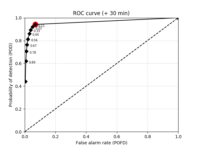
Verification

Pysteps includes a number of verification metrics to help users to analyze the general characteristics of the nowcasts in terms of consistency and quality (or goodness). Here, we will verify our probabilistic forecasts using the ROC curve, reliability diagrams, and rank histograms, as implemented in the verification module of pysteps.

# Find the files containing the verifying observations
fns = io.archive.find_by_date(
    date,
    root_path,
    path_fmt,
    fn_pattern,
    fn_ext,
    timestep,
    0,
    num_next_files=n_leadtimes,
)

# Read the observations
R_o, _, metadata_o = io.read_timeseries(fns, importer, **importer_kwargs)

# Convert to mm/h
R_o, metadata_o = conversion.to_rainrate(R_o, metadata_o)

# Upscale data to 2 km
R_o, metadata_o = dimension.aggregate_fields_space(R_o, metadata_o, 2000)

# Compute the verification for the last lead time

# compute the exceedance probability of 0.1 mm/h from the ensemble
P_f = ensemblestats.excprob(R_f[:, -1, :, :], 0.1, ignore_nan=True)

# compute and plot the ROC curve
roc = verification.ROC_curve_init(0.1, n_prob_thrs=10)
verification.ROC_curve_accum(roc, P_f, R_o[-1, :, :])
fig, ax = subplots()
verification.plot_ROC(roc, ax, opt_prob_thr=True)
ax.set_title("ROC curve (+ %i min)" % (n_leadtimes * timestep))

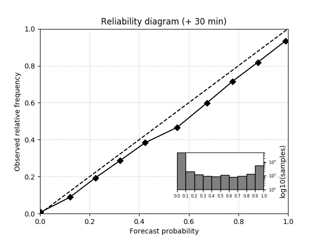
# compute and plot the reliability diagram
reldiag = verification.reldiag_init(0.1)
verification.reldiag_accum(reldiag, P_f, R_o[-1, :, :])
fig, ax = subplots()
verification.plot_reldiag(reldiag, ax)
ax.set_title("Reliability diagram (+ %i min)" % (n_leadtimes * timestep))

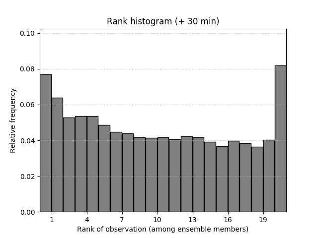
# compute and plot the rank histogram
rankhist = verification.rankhist_init(R_f.shape[0], 0.1)
verification.rankhist_accum(rankhist, R_f[:, -1, :, :], R_o[-1, :, :])
fig, ax = subplots()
verification.plot_rankhist(rankhist, ax)
ax.set_title("Rank histogram (+ %i min)" % (n_leadtimes * timestep))

# sphinx_gallery_thumbnail_number = 5

• 
• 
•