Linear blending

This tutorial shows how to construct a simple linear blending between a STEPS ensemble nowcast and a Numerical Weather Prediction (NWP) rainfall forecast. The used datasets are from the Bureau of Meteorology, Australia.

import os
from datetime import datetime

from matplotlib import pyplot as plt

import pysteps
from pysteps import io, rcparams, blending
from pysteps.visualization import plot_precip_field

Read the radar images and the NWP forecast

First, we import a sequence of 3 images of 10-minute radar composites and the corresponding NWP rainfall forecast that was available at that time.

You need the pysteps-data archive downloaded and the pystepsrc file configured with the data_source paths pointing to data folders. Additionally, the pysteps-nwp-importers plugin needs to be installed, see https://github.com/pySTEPS/pysteps-nwp-importers.

# Selected case
date_radar = datetime.strptime("202010310400", "%Y%m%d%H%M")
# The last NWP forecast was issued at 00:00
date_nwp = datetime.strptime("202010310000", "%Y%m%d%H%M")
radar_data_source = rcparams.data_sources["bom"]
nwp_data_source = rcparams.data_sources["bom_nwp"]

Load the data from the archive

root_path = radar_data_source["root_path"]
path_fmt = "prcp-c10/66/%Y/%m/%d"
fn_pattern = "66_%Y%m%d_%H%M00.prcp-c10"
fn_ext = radar_data_source["fn_ext"]
importer_name = radar_data_source["importer"]
importer_kwargs = radar_data_source["importer_kwargs"]
timestep = 10.0

# Find the radar files in the archive
fns = io.find_by_date(
    date_radar, root_path, path_fmt, fn_pattern, fn_ext, timestep, num_prev_files=2
)

# Read the radar composites
importer = io.get_method(importer_name, "importer")
radar_precip, _, radar_metadata = io.read_timeseries(fns, importer, **importer_kwargs)

# Import the NWP data
filename = os.path.join(
    nwp_data_source["root_path"],
    datetime.strftime(date_nwp, nwp_data_source["path_fmt"]),
    datetime.strftime(date_nwp, nwp_data_source["fn_pattern"])
    + "."
    + nwp_data_source["fn_ext"],
)

nwp_importer = io.get_method("bom_nwp", "importer")
nwp_precip, _, nwp_metadata = nwp_importer(filename)

# Only keep the NWP forecasts from the last radar observation time (2020-10-31 04:00)
# End of the forecast is 18 time steps (+3 hours) in advance.
precip_nwp = nwp_precip[24:43, :, :]

Out:

Rainfall values are accumulated. Disaggregating by time step

Pre-processing steps

# Make sure the units are in mm/h
converter = pysteps.utils.get_method("mm/h")
radar_precip, radar_metadata = converter(radar_precip, radar_metadata)
precip_nwp, nwp_metadata = converter(precip_nwp, nwp_metadata)

# Threshold the data
radar_precip[radar_precip < 0.1] = 0.0
precip_nwp[precip_nwp < 0.1] = 0.0

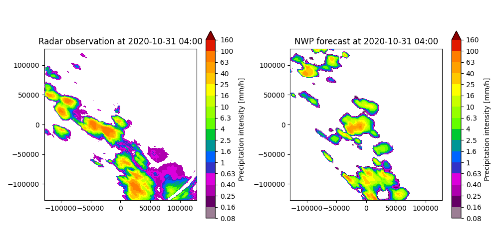
# Plot the radar rainfall field and the first time step of the NWP forecast.
# For the initial time step (t=0), the NWP rainfall forecast is not that different
# from the observed radar rainfall, but it misses some of the locations and
# shapes of the observed rainfall fields. Therefore, the NWP rainfall forecast will
# initially get a low weight in the blending process.
date_str = datetime.strftime(date_radar, "%Y-%m-%d %H:%M")
plt.figure(figsize=(10, 5))
plt.subplot(121)
plot_precip_field(
    radar_precip[-1, :, :],
    geodata=radar_metadata,
    title=f"Radar observation at {date_str}",
)
plt.subplot(122)
plot_precip_field(
    precip_nwp[0, :, :], geodata=nwp_metadata, title=f"NWP forecast at {date_str}"
)
plt.tight_layout()
plt.show()

# Only keep the NWP forecasts from 2020-10-31 04:05 onwards, because the first
# forecast lead time starts at 04:05.
precip_nwp = precip_nwp[1:]

# Transform the radar data to dB - this transformation is useful for the motion
# field estimation and the subsequent nowcasts. The NWP forecast is not
# transformed, because the linear blending code sets everything back in mm/h
# after the nowcast.
transformer = pysteps.utils.get_method("dB")
radar_precip, radar_metadata = transformer(radar_precip, radar_metadata, threshold=0.1)

Determine the velocity field for the radar rainfall nowcast

oflow_method = pysteps.motion.get_method("lucaskanade")
velocity_radar = oflow_method(radar_precip)

The linear blending of nowcast and NWP rainfall forecast

# Calculate the blended precipitation field
precip_blended = blending.linear_blending.forecast(
    precip=radar_precip[-1, :, :],
    precip_metadata=radar_metadata,
    velocity=velocity_radar,
    timesteps=18,
    timestep=10,
    nowcast_method="extrapolation",  # simple advection nowcast
    precip_nwp=precip_nwp,
    precip_nwp_metadata=nwp_metadata,
    start_blending=60,  # in minutes (this is an arbritrary choice)
    end_blending=120,  # in minutes (this is an arbritrary choice)
)

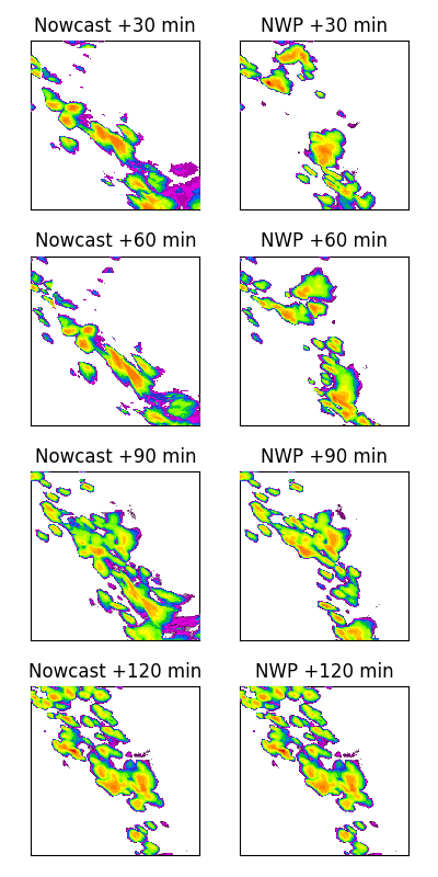
Visualize the output

The linear blending starts at 60 min, so during the first 60 minutes the blended forecast only consists of the extrapolation forecast (consisting of an extrapolation nowcast). Between 60 and 120 min, the NWP forecast gradually gets more weight, whereas the extrapolation forecasts gradually gets less weight. After 120 min, the blended forecast entirely consists of the NWP rainfall forecast.

fig = plt.figure(figsize=(4, 8))

leadtimes_min = [30, 60, 90, 120]
n_leadtimes = len(leadtimes_min)
for n, leadtime in enumerate(leadtimes_min):

    # Nowcast with blending into NWP
    plt.subplot(n_leadtimes, 2, n * 2 + 1)
    plot_precip_field(
        precip_blended[int(leadtime / timestep) - 1, :, :],
        geodata=radar_metadata,
        title=f"Nowcast +{leadtime} min",
        axis="off",
        colorbar=False,
    )

    # Raw NWP forecast
    plt.subplot(n_leadtimes, 2, n * 2 + 2)
    plot_precip_field(
        precip_nwp[int(leadtime / timestep) - 1, :, :],
        geodata=nwp_metadata,
        title=f"NWP +{leadtime} min",
        axis="off",
        colorbar=False,
    )

plt.tight_layout()
plt.show()