Blended forecast

This tutorial shows how to construct a blended forecast from an ensemble nowcast using the STEPS approach and a Numerical Weather Prediction (NWP) rainfall forecast. The used datasets are from the Bureau of Meteorology, Australia.

import os
from datetime import datetime

import numpy as np
from matplotlib import pyplot as plt

import pysteps
from pysteps import io, rcparams, blending, nowcasts
from pysteps.visualization import plot_precip_field

Read the radar images and the NWP forecast

First, we import a sequence of 3 images of 10-minute radar composites and the corresponding NWP rainfall forecast that was available at that time.

You need the pysteps-data archive downloaded and the pystepsrc file configured with the data_source paths pointing to data folders. Additionally, the pysteps-nwp-importers plugin needs to be installed, see pySTEPS/pysteps-nwp-importers.

# Selected case
date_radar = datetime.strptime("202010310400", "%Y%m%d%H%M")
# The last NWP forecast was issued at 00:00
date_nwp = datetime.strptime("202010310000", "%Y%m%d%H%M")
radar_data_source = rcparams.data_sources["bom"]
nwp_data_source = rcparams.data_sources["bom_nwp"]

Load the data from the archive

root_path = radar_data_source["root_path"]
path_fmt = "prcp-c10/66/%Y/%m/%d"
fn_pattern = "66_%Y%m%d_%H%M00.prcp-c10"
fn_ext = radar_data_source["fn_ext"]
importer_name = radar_data_source["importer"]
importer_kwargs = radar_data_source["importer_kwargs"]
timestep = 10.0

# Find the radar files in the archive
fns = io.find_by_date(
    date_radar, root_path, path_fmt, fn_pattern, fn_ext, timestep, num_prev_files=2
)

# Read the radar composites
importer = io.get_method(importer_name, "importer")
radar_precip, _, radar_metadata = io.read_timeseries(fns, importer, **importer_kwargs)

# Import the NWP data
filename = os.path.join(
    nwp_data_source["root_path"],
    datetime.strftime(date_nwp, nwp_data_source["path_fmt"]),
    datetime.strftime(date_nwp, nwp_data_source["fn_pattern"])
    + "."
    + nwp_data_source["fn_ext"],
)

nwp_importer = io.get_method("bom_nwp", "importer")
nwp_precip, _, nwp_metadata = nwp_importer(filename)

# Only keep the NWP forecasts from the last radar observation time (2020-10-31 04:00)
# onwards

nwp_precip = nwp_precip[24:43, :, :]

Rainfall values are accumulated. Disaggregating by time step

Pre-processing steps

# Make sure the units are in mm/h
converter = pysteps.utils.get_method("mm/h")
radar_precip, radar_metadata = converter(radar_precip, radar_metadata)
nwp_precip, nwp_metadata = converter(nwp_precip, nwp_metadata)

# Threshold the data
radar_precip[radar_precip < 0.1] = 0.0
nwp_precip[nwp_precip < 0.1] = 0.0

# Plot the radar rainfall field and the first time step of the NWP forecast.
date_str = datetime.strftime(date_radar, "%Y-%m-%d %H:%M")
plt.figure(figsize=(10, 5))
plt.subplot(121)
plot_precip_field(
    radar_precip[-1, :, :],
    geodata=radar_metadata,
    title=f"Radar observation at {date_str}",
    colorscale="STEPS-NL",
)
plt.subplot(122)
plot_precip_field(
    nwp_precip[0, :, :],
    geodata=nwp_metadata,
    title=f"NWP forecast at {date_str}",
    colorscale="STEPS-NL",
)
plt.tight_layout()
plt.show()

# transform the data to dB
transformer = pysteps.utils.get_method("dB")
radar_precip, radar_metadata = transformer(radar_precip, radar_metadata, threshold=0.1)
nwp_precip, nwp_metadata = transformer(nwp_precip, nwp_metadata, threshold=0.1)

# r_nwp has to be four dimentional (n_models, time, y, x).
# If we only use one model:
if nwp_precip.ndim == 3:
    nwp_precip = nwp_precip[None, :]

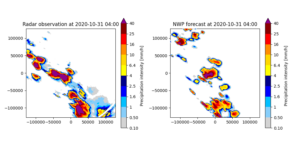
For the initial time step (t=0), the NWP rainfall forecast is not that different from the observed radar rainfall, but it misses some of the locations and shapes of the observed rainfall fields. Therefore, the NWP rainfall forecast will initially get a low weight in the blending process.

Determine the velocity fields

oflow_method = pysteps.motion.get_method("lucaskanade")

# First for the radar images
velocity_radar = oflow_method(radar_precip)

# Then for the NWP forecast
velocity_nwp = []
# Loop through the models
for n_model in range(nwp_precip.shape[0]):
    # Loop through the timesteps. We need two images to construct a motion
    # field, so we can start from timestep 1. Timestep 0 will be the same
    # as timestep 1.
    _v_nwp_ = []
    for t in range(1, nwp_precip.shape[1]):
        v_nwp_ = oflow_method(nwp_precip[n_model, t - 1 : t + 1, :])
        _v_nwp_.append(v_nwp_)
        v_nwp_ = None
    # Add the velocity field at time step 1 to time step 0.
    _v_nwp_ = np.insert(_v_nwp_, 0, _v_nwp_[0], axis=0)
    velocity_nwp.append(_v_nwp_)
velocity_nwp = np.stack(velocity_nwp)

The blended forecast

precip_forecast = blending.steps.forecast(
    precip=radar_precip,
    precip_models=nwp_precip,
    velocity=velocity_radar,
    velocity_models=velocity_nwp,
    timesteps=18,
    timestep=timestep,
    issuetime=date_radar,
    n_ens_members=1,
    precip_thr=radar_metadata["threshold"],
    kmperpixel=radar_metadata["xpixelsize"] / 1000.0,
    noise_stddev_adj="auto",
    vel_pert_method=None,
)

# Transform the data back into mm/h
precip_forecast, _ = converter(precip_forecast, radar_metadata)
radar_precip_mmh, _ = converter(radar_precip, radar_metadata)
nwp_precip_mmh, _ = converter(nwp_precip, nwp_metadata)

STEPS blending
==============

Inputs
------
forecast issue time:         2020-10-31T04:00:00
input dimensions:            512x512
km/pixel:                    0.5
time step:                   10.0 minutes

NWP and blending inputs
-----------------------
number of (NWP) models:      1
blend (NWP) model members:   False
decompose (NWP) models:      yes

Methods
-------
extrapolation:               semilagrangian
bandpass filter:             gaussian
decomposition:               fft
nowcasting algorithm:        steps
noise generator:             nonparametric
noise adjustment:            yes
velocity perturbator:        None
blending weights method:     bps
conditional statistics:      no
precip. mask method:         incremental
probability matching:        cdf
FFT method:                  numpy
domain:                      spatial

Parameters
----------
time steps:                  [0, 1, 2, 3, 4, 5, 6, 7, 8, 9, 10, 11, 12, 13, 14, 15, 16, 17, 18]
ensemble size:               1
parallel threads:            1
number of cascade levels:    6
order of the AR(p) model:    2
precip. intensity threshold: -10.0
no-rain fraction threshold for radar: 0.0

Blended nowcast components initialized successfully.
Rain fraction is: 0.20020675659179688, while minimum fraction is 0.0
Rain fraction is: 0.19766315660978617, while minimum fraction is 0.0
Computing noise adjustment coefficients... done.
noise std. dev. coeffs:   [1.00477124 1.22096262 1.02495162 0.82721102 0.6162069  0.54739187]
************************************************
* Correlation coefficients for cascade levels: *
************************************************
-----------------------------------------
| Level |     Lag-1     |     Lag-2     |
-----------------------------------------
| 1     | 0.994780      | 0.983034      |
-----------------------------------------
| 2     | 0.946583      | 0.848484      |
-----------------------------------------
| 3     | 0.754590      | 0.539837      |
-----------------------------------------
| 4     | 0.351598      | 0.136960      |
-----------------------------------------
| 5     | 0.160575      | 0.133259      |
-----------------------------------------
| 6     | 0.138575      | 0.154904      |
-----------------------------------------
****************************************
* AR(p) parameters for cascade levels: *
****************************************
------------------------------------------------------
| Level |    Phi-1     |    Phi-2     |    Phi-0     |
------------------------------------------------------
| 1     | 1.620686     | -0.629192    | 0.079316     |
------------------------------------------------------
| 2     | 1.379307     | -0.457143    | 0.286795     |
------------------------------------------------------
| 3     | 0.806409     | -0.068672    | 0.654647     |
------------------------------------------------------
| 4     | 0.346247     | 0.015220     | 0.936043     |
------------------------------------------------------
| 5     | 0.142861     | 0.110319     | 0.980999     |
------------------------------------------------------
| 6     | 0.119402     | 0.138358     | 0.980827     |
------------------------------------------------------
Starting blended nowcast computation.
Computing nowcast for time step 1... done.
Computing nowcast for time step 2... done.
Computing nowcast for time step 3... done.
Computing nowcast for time step 4... done.
Computing nowcast for time step 5... done.
Computing nowcast for time step 6... done.
Computing nowcast for time step 7... done.
Computing nowcast for time step 8... done.
Computing nowcast for time step 9... done.
Computing nowcast for time step 10... done.
Computing nowcast for time step 11... done.
Computing nowcast for time step 12... done.
Computing nowcast for time step 13... done.
Computing nowcast for time step 14... done.
Computing nowcast for time step 15... done.
Computing nowcast for time step 16... done.
Computing nowcast for time step 17... done.
Computing nowcast for time step 18... done.

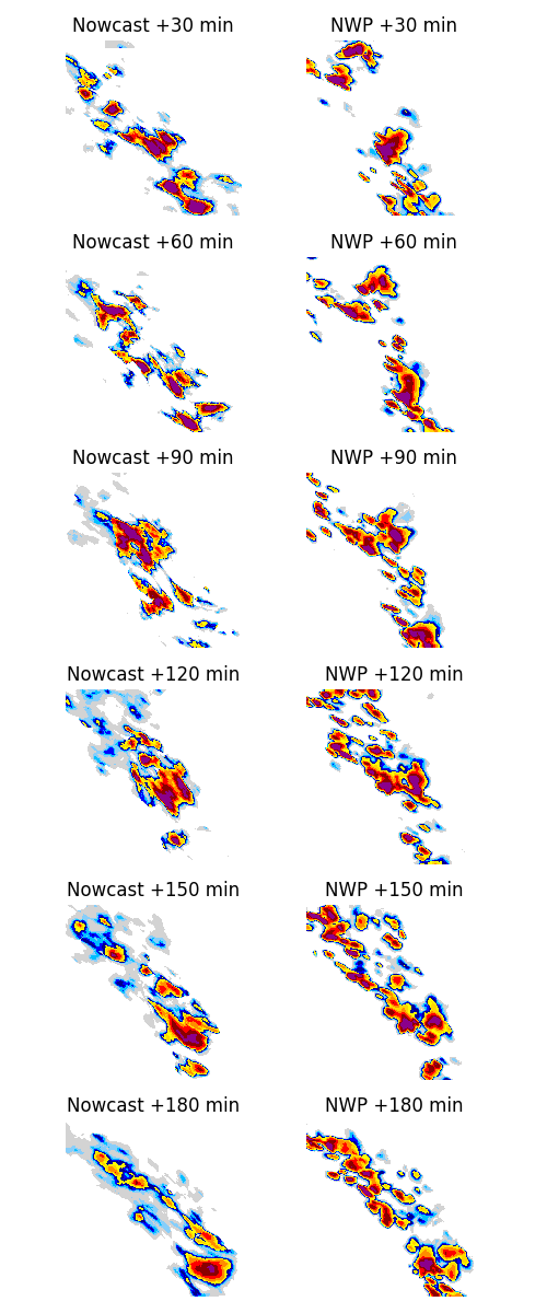
Visualize the output

The NWP rainfall forecast has a lower weight than the radar-based extrapolation forecast at the issue time of the forecast (+0 min). Therefore, the first time steps consist mostly of the extrapolation. However, near the end of the forecast (+180 min), the NWP share in the blended forecast has become more important and the forecast starts to resemble the NWP forecast more.

fig = plt.figure(figsize=(5, 12))

leadtimes_min = [30, 60, 90, 120, 150, 180]
n_leadtimes = len(leadtimes_min)
for n, leadtime in enumerate(leadtimes_min):
    # Nowcast with blending into NWP
    ax1 = plt.subplot(n_leadtimes, 2, n * 2 + 1)
    plot_precip_field(
        precip_forecast[0, int(leadtime / timestep) - 1, :, :],
        geodata=radar_metadata,
        title=f"Nowcast +{leadtime} min",
        axis="off",
        colorscale="STEPS-NL",
        colorbar=False,
    )
    ax1.axis("off")

    # Raw NWP forecast
    plt.subplot(n_leadtimes, 2, n * 2 + 2)
    ax2 = plot_precip_field(
        nwp_precip_mmh[0, int(leadtime / timestep) - 1, :, :],
        geodata=nwp_metadata,
        title=f"NWP +{leadtime} min",
        axis="off",
        colorscale="STEPS-NL",
        colorbar=False,
    )
    ax2.axis("off")

plt.tight_layout()
plt.show()

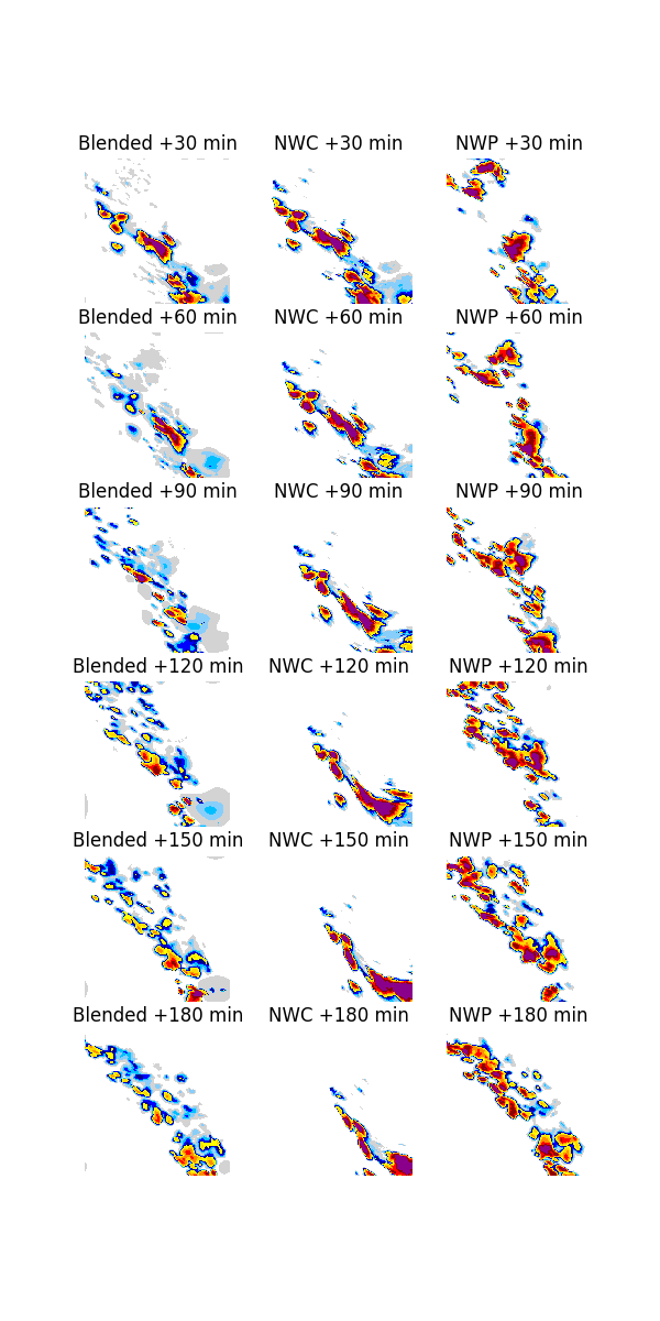
It is also possible to blend a deterministic or probabilistic external nowcast (e.g. a pre-made nowcast or a deterministic AI-based nowcast) with NWP using the STEPS algorithm. In that case, we add a precip_nowcast to blending.steps.forecast. By providing an external nowcast, the STEPS blending method will omit the autoregression and advection step for the extrapolation cascade and use the existing external nowcast instead (which will thus be decomposed into multiplicative cascades!). The weights determination and possible post-processings steps will remain the same.

Start with creating an external nowcast

# We go for a simple advection-only nowcast for the example, but this setup can
# be replaced with any external deterministic or probabilistic nowcast.
extrapolate = nowcasts.get_method("extrapolation")
radar_precip_to_advect = radar_precip.copy()
radar_metadata_to_advect = radar_metadata.copy()

# Make sure the data has no nans
radar_precip_to_advect[~np.isfinite(radar_precip_to_advect)] = -15
radar_precip_to_advect = radar_precip_to_advect.data

# Create the extrapolation
fc_lagrangian_extrapolation = extrapolate(
    radar_precip_to_advect[-1, :, :], velocity_radar, 18
)

# Insert an additional timestep at the start, as t0, which is the same as the current first slice.
fc_lagrangian_extrapolation = np.insert(
    fc_lagrangian_extrapolation, 0, fc_lagrangian_extrapolation[0:1, :, :], axis=0
)
fc_lagrangian_extrapolation[~np.isfinite(fc_lagrangian_extrapolation)] = (
    radar_metadata_to_advect["zerovalue"]
)

Blend the external nowcast with NWP - deterministic mode

precip_forecast = blending.steps.forecast(
    precip=radar_precip,
    precip_nowcast=np.array(
        [fc_lagrangian_extrapolation]
    ),  # Add an extra dimension, becuase precip_nowcast has to be 4-dimensional
    precip_models=nwp_precip,
    velocity=velocity_radar,
    velocity_models=velocity_nwp,
    timesteps=18,
    timestep=timestep,
    issuetime=date_radar,
    n_ens_members=1,
    precip_thr=radar_metadata["threshold"],
    kmperpixel=radar_metadata["xpixelsize"] / 1000.0,
    noise_stddev_adj="auto",
    vel_pert_method=None,
    nowcasting_method="external_nowcast",
    noise_method=None,
    probmatching_method=None,
    mask_method=None,
    weights_method="bps",
)

# Transform the data back into mm/h
precip_forecast, _ = converter(precip_forecast, radar_metadata)
radar_precip_mmh, _ = converter(radar_precip, radar_metadata)
fc_lagrangian_extrapolation_mmh, _ = converter(
    fc_lagrangian_extrapolation, radar_metadata_to_advect
)
nwp_precipfc_lagrangian_extrapolation_mmh_mmh, _ = converter(nwp_precip, nwp_metadata)

STEPS blending
==============

Inputs
------
forecast issue time:         2020-10-31T04:00:00
input dimensions:            512x512
input dimensions pre-computed nowcast:            512x512
km/pixel:                    0.5
time step:                   10.0 minutes

NWP and blending inputs
-----------------------
number of (NWP) models:      1
blend (NWP) model members:   False
decompose (NWP) models:      yes

Methods
-------
extrapolation:               semilagrangian
bandpass filter:             gaussian
decomposition:               fft
nowcasting algorithm:        external_nowcast
noise generator:             None
noise adjustment:            yes
velocity perturbator:        None
blending weights method:     bps
conditional statistics:      no
precip. mask method:         None
probability matching:        None
FFT method:                  numpy
domain:                      spatial

Parameters
----------
time steps:                  [0, 1, 2, 3, 4, 5, 6, 7, 8, 9, 10, 11, 12, 13, 14, 15, 16, 17, 18]
ensemble size:               1
parallel threads:            1
number of cascade levels:    6
order of the AR(p) model:    2
no-rain fraction threshold for radar: 0.0

Blended nowcast components initialized successfully.
Rain fraction is: 0.20020675659179688, while minimum fraction is 0.0
Rain fraction is: 0.19766315660978617, while minimum fraction is 0.0
************************************************
* Correlation coefficients for cascade levels: *
************************************************
-----------------------------------------
| Level |     Lag-1     |     Lag-2     |
-----------------------------------------
| 1     | 0.994780      | 0.983034      |
-----------------------------------------
| 2     | 0.946583      | 0.848484      |
-----------------------------------------
| 3     | 0.754590      | 0.539837      |
-----------------------------------------
| 4     | 0.351598      | 0.136960      |
-----------------------------------------
| 5     | 0.160575      | 0.133259      |
-----------------------------------------
| 6     | 0.138575      | 0.154904      |
-----------------------------------------
****************************************
* AR(p) parameters for cascade levels: *
****************************************
------------------------------------------------------
| Level |    Phi-1     |    Phi-2     |    Phi-0     |
------------------------------------------------------
| 1     | 1.620686     | -0.629192    | 0.079316     |
------------------------------------------------------
| 2     | 1.379307     | -0.457143    | 0.286795     |
------------------------------------------------------
| 3     | 0.806409     | -0.068672    | 0.654647     |
------------------------------------------------------
| 4     | 0.346247     | 0.015220     | 0.936043     |
------------------------------------------------------
| 5     | 0.142861     | 0.110319     | 0.980999     |
------------------------------------------------------
| 6     | 0.119402     | 0.138358     | 0.980827     |
------------------------------------------------------
Starting blended nowcast computation.
Computing nowcast for time step 1... done.
Computing nowcast for time step 2... done.
Computing nowcast for time step 3... done.
Computing nowcast for time step 4... done.
Computing nowcast for time step 5... done.
Computing nowcast for time step 6... done.
Computing nowcast for time step 7... done.
Computing nowcast for time step 8... done.
Computing nowcast for time step 9... done.
Computing nowcast for time step 10... done.
Computing nowcast for time step 11... done.
Computing nowcast for time step 12... done.
Computing nowcast for time step 13... done.
Computing nowcast for time step 14... done.
Computing nowcast for time step 15... done.
Computing nowcast for time step 16... done.
Computing nowcast for time step 17... done.
Computing nowcast for time step 18... done.

Visualize the output

The NWP rainfall forecast has a lower weight than the radar-based extrapolation forecast at the issue time of the forecast (+0 min). Therefore, the first time steps consist mostly of the extrapolation. However, near the end of the forecast (+180 min), the NWP share in the blended forecast has become more important and the forecast starts to resemble the NWP forecast more.

fig = plt.figure(figsize=(6, 12))

leadtimes_min = [30, 60, 90, 120, 150, 180]
n_leadtimes = len(leadtimes_min)

for n, leadtime in enumerate(leadtimes_min):
    idx = int(leadtime / timestep) - 1

    # Blended nowcast
    ax1 = plt.subplot(n_leadtimes, 3, n * 3 + 1)
    plot_precip_field(
        precip_forecast[0, idx, :, :],
        geodata=radar_metadata,
        title=f"Blended +{leadtime} min",
        axis="off",
        colorscale="STEPS-NL",
        colorbar=False,
    )
    ax1.axis("off")

    # Raw extrapolated nowcast
    ax2 = plt.subplot(n_leadtimes, 3, n * 3 + 2)
    plot_precip_field(
        fc_lagrangian_extrapolation_mmh[idx, :, :],
        geodata=radar_metadata,
        title=f"NWC +{leadtime} min",
        axis="off",
        colorscale="STEPS-NL",
        colorbar=False,
    )
    ax2.axis("off")

    # Raw NWP forecast
    plt.subplot(n_leadtimes, 3, n * 3 + 3)
    ax3 = plot_precip_field(
        nwp_precip_mmh[0, idx, :, :],
        geodata=nwp_metadata,
        title=f"NWP +{leadtime} min",
        axis="off",
        colorscale="STEPS-NL",
        colorbar=False,
    )
    ax3.axis("off")

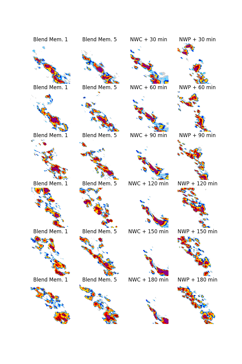
Blend the external nowcast with NWP - ensemble mode

precip_forecast = blending.steps.forecast(
    precip=radar_precip,
    precip_nowcast=np.array(
        [fc_lagrangian_extrapolation]
    ),  # Add an extra dimension, becuase precip_nowcast has to be 4-dimensional
    precip_models=nwp_precip,
    velocity=velocity_radar,
    velocity_models=velocity_nwp,
    timesteps=18,
    timestep=timestep,
    issuetime=date_radar,
    n_ens_members=5,
    precip_thr=radar_metadata["threshold"],
    kmperpixel=radar_metadata["xpixelsize"] / 1000.0,
    noise_stddev_adj="auto",
    vel_pert_method=None,
    nowcasting_method="external_nowcast",
    noise_method="nonparametric",
    probmatching_method="cdf",
    mask_method="incremental",
    weights_method="bps",
)

# Transform the data back into mm/h
precip_forecast, _ = converter(precip_forecast, radar_metadata)
radar_precip_mmh, _ = converter(radar_precip, radar_metadata)
fc_lagrangian_extrapolation_mmh, _ = converter(
    fc_lagrangian_extrapolation, radar_metadata_to_advect
)
nwp_precipfc_lagrangian_extrapolation_mmh_mmh, _ = converter(nwp_precip, nwp_metadata)

STEPS blending
==============

Inputs
------
forecast issue time:         2020-10-31T04:00:00
input dimensions:            512x512
input dimensions pre-computed nowcast:            512x512
km/pixel:                    0.5
time step:                   10.0 minutes

NWP and blending inputs
-----------------------
number of (NWP) models:      1
blend (NWP) model members:   False
decompose (NWP) models:      yes

Methods
-------
extrapolation:               semilagrangian
bandpass filter:             gaussian
decomposition:               fft
nowcasting algorithm:        external_nowcast
noise generator:             nonparametric
noise adjustment:            yes
velocity perturbator:        None
blending weights method:     bps
conditional statistics:      no
precip. mask method:         incremental
probability matching:        cdf
FFT method:                  numpy
domain:                      spatial

Parameters
----------
time steps:                  [0, 1, 2, 3, 4, 5, 6, 7, 8, 9, 10, 11, 12, 13, 14, 15, 16, 17, 18]
ensemble size:               5
parallel threads:            1
number of cascade levels:    6
order of the AR(p) model:    2
precip. intensity threshold: -10.0
no-rain fraction threshold for radar: 0.0

Blended nowcast components initialized successfully.
Rain fraction is: 0.20020675659179688, while minimum fraction is 0.0
Rain fraction is: 0.19766315660978617, while minimum fraction is 0.0
Computing noise adjustment coefficients... done.
noise std. dev. coeffs:   [0.96569561 1.17933695 1.00143589 0.80243268 0.59268058 0.52357645]
************************************************
* Correlation coefficients for cascade levels: *
************************************************
-----------------------------------------
| Level |     Lag-1     |     Lag-2     |
-----------------------------------------
| 1     | 0.994780      | 0.983034      |
-----------------------------------------
| 2     | 0.946583      | 0.848484      |
-----------------------------------------
| 3     | 0.754590      | 0.539837      |
-----------------------------------------
| 4     | 0.351598      | 0.136960      |
-----------------------------------------
| 5     | 0.160575      | 0.133259      |
-----------------------------------------
| 6     | 0.138575      | 0.154904      |
-----------------------------------------
****************************************
* AR(p) parameters for cascade levels: *
****************************************
------------------------------------------------------
| Level |    Phi-1     |    Phi-2     |    Phi-0     |
------------------------------------------------------
| 1     | 1.620686     | -0.629192    | 0.079316     |
------------------------------------------------------
| 2     | 1.379307     | -0.457143    | 0.286795     |
------------------------------------------------------
| 3     | 0.806409     | -0.068672    | 0.654647     |
------------------------------------------------------
| 4     | 0.346247     | 0.015220     | 0.936043     |
------------------------------------------------------
| 5     | 0.142861     | 0.110319     | 0.980999     |
------------------------------------------------------
| 6     | 0.119402     | 0.138358     | 0.980827     |
------------------------------------------------------
Starting blended nowcast computation.
Repeating the NWP model for all ensemble members
Repeating the nowcast for all ensemble members
Computing nowcast for time step 1... Repeating the NWP model for all ensemble members
done.
Computing nowcast for time step 2... Repeating the NWP model for all ensemble members
done.
Computing nowcast for time step 3... Repeating the NWP model for all ensemble members
done.
Computing nowcast for time step 4... Repeating the NWP model for all ensemble members
done.
Computing nowcast for time step 5... Repeating the NWP model for all ensemble members
done.
Computing nowcast for time step 6... Repeating the NWP model for all ensemble members
done.
Computing nowcast for time step 7... Repeating the NWP model for all ensemble members
done.
Computing nowcast for time step 8... Repeating the NWP model for all ensemble members
done.
Computing nowcast for time step 9... Repeating the NWP model for all ensemble members
done.
Computing nowcast for time step 10... Repeating the NWP model for all ensemble members
done.
Computing nowcast for time step 11... Repeating the NWP model for all ensemble members
done.
Computing nowcast for time step 12... Repeating the NWP model for all ensemble members
done.
Computing nowcast for time step 13... Repeating the NWP model for all ensemble members
done.
Computing nowcast for time step 14... Repeating the NWP model for all ensemble members
done.
Computing nowcast for time step 15... Repeating the NWP model for all ensemble members
done.
Computing nowcast for time step 16... Repeating the NWP model for all ensemble members
done.
Computing nowcast for time step 17... Repeating the NWP model for all ensemble members
done.
Computing nowcast for time step 18... Repeating the NWP model for all ensemble members
done.

Visualize the output

fig = plt.figure(figsize=(8, 12))

leadtimes_min = [30, 60, 90, 120, 150, 180]
n_leadtimes = len(leadtimes_min)

for n, leadtime in enumerate(leadtimes_min):
    idx = int(leadtime / timestep) - 1

    # Blended nowcast member 1
    ax1 = plt.subplot(n_leadtimes, 4, n * 4 + 1)
    plot_precip_field(
        precip_forecast[0, idx, :, :],
        geodata=radar_metadata,
        title="Blend Mem. 1",
        axis="off",
        colorscale="STEPS-NL",
        colorbar=False,
    )
    ax1.axis("off")

    # Blended nowcast member 5
    ax2 = plt.subplot(n_leadtimes, 4, n * 4 + 2)
    plot_precip_field(
        precip_forecast[4, idx, :, :],
        geodata=radar_metadata,
        title="Blend Mem. 5",
        axis="off",
        colorscale="STEPS-NL",
        colorbar=False,
    )
    ax2.axis("off")

    # Raw extrapolated nowcast
    ax3 = plt.subplot(n_leadtimes, 4, n * 4 + 3)
    plot_precip_field(
        fc_lagrangian_extrapolation_mmh[idx, :, :],
        geodata=radar_metadata,
        title=f"NWC + {leadtime} min",
        axis="off",
        colorscale="STEPS-NL",
        colorbar=False,
    )
    ax3.axis("off")

    # Raw NWP forecast
    ax4 = plt.subplot(n_leadtimes, 4, n * 4 + 4)
    plot_precip_field(
        nwp_precip_mmh[0, idx, :, :],
        geodata=nwp_metadata,
        title=f"NWP + {leadtime} min",
        axis="off",
        colorscale="STEPS-NL",
        colorbar=False,
    )
    ax4.axis("off")

plt.show()

print("Done.")

Done.

References

Bowler, N. E., and C. E. Pierce, and A. W. Seed. 2004. “STEPS: A probabilistic precipitation forecasting scheme which merges an extrapolation nowcast with downscaled NWP.” Forecasting Research Technical Report No. 433. Wallingford, UK.

Bowler, N. E., and C. E. Pierce, and A. W. Seed. 2006. “STEPS: A probabilistic precipitation forecasting scheme which merges an extrapolation nowcast with downscaled NWP.” Quarterly Journal of the Royal Meteorological Society 132(16): 2127-2155. https://doi.org/10.1256/qj.04.100

Seed, A. W., and C. E. Pierce, and K. Norman. 2013. “Formulation and evaluation of a scale decomposition-based stochastic precipitation nowcast scheme.” Water Resources Research 49(10): 6624-664. https://doi.org/10.1002/wrcr.20536

Imhoff, R.O., L. De Cruz, W. Dewettinck, C.C. Brauer, R. Uijlenhoet, K-J. van Heeringen, C. Velasco-Forero, D. Nerini, M. Van Ginderachter, and A.H. Weerts. 2023. “Scale-dependent blending of ensemble rainfall nowcasts and NWP in the open-source pysteps library”. Quarterly Journal of the Royal Meteorological Society 149(753): 1-30. https://doi.org/10.1002/qj.4461